
Questions:
- How do I find sequence variants between my sample and a reference genome?
Objectives:
- Understand the steps involved in variant calling.
- Describe the types of data formats encountered during variant calling.
- Use command line tools to perform variant calling.
It’s always good to acknowledge the people who create these great lessons. This one is adapted from Data Carpentry “Wrangling Genomics” We mentioned before that we are working with files from a long-term evolution study of an E. coli population (designated Ara-3). The basic concept is to understand how genomes can evolve over time, in particular to understand if evolution happens in “jumps” or if it is essentially a consitent force (that might be measured!). Now that we have looked at our data to make sure that it is high quality, and removed low-quality base calls, we can perform variant calling to see how the population changed over time. We care how this population changed relative to the original population, E. coli strain REL606. Therefore, we will align each of our samples to the E. coli REL606 reference genome, and see what differences exist in our reads versus the genome.
What are variants?
The NCI Dictionary of Genetics Terms defines a genetic variant as “An alteration in the most common DNA nucleotide sequence. The term variant can be used to describe an alteration that may be benign, pathogenic, or of unknown significance. The term variant is increasingly being used in place of the term mutation.”
Genetic variation and mutations are related, but not the same. The three primary causes for genetic variation are horizontal gene transfer, recombination during sexual reproduction, and mutations. For mutations, there are three primary types: Insertions, Deletions, and Base Substitutions. The common term for these mutation types is “indels”. Most software that claims to measure “variants”, actually measure “indels”. Also, to define an indel as a “variant”, one must compare the indels to a “reference” sequence. We don’t need to know all the technical details of evolution, but it’s good to understand that this experiment is measuring changes in the genome over time, using the REL606 genome as the reference.
Alignment to a reference genome
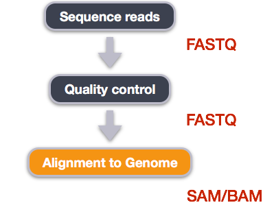
We perform read alignment or mapping to determine where in the genome our reads originated from. There are a number of tools to choose from and, while there is no gold standard, there are some tools that are better suited for particular NGS analyses. We will be using the Burrows Wheeler Aligner (BWA), which is a software package for mapping low-divergent sequences against a large reference genome.
The alignment process consists of two steps:
- Indexing the reference genome
- Aligning the reads to the reference genome
Setting up the data
First we download the reference genome for E. coli REL606. Although we could copy or move the file with cp or mv, most genomics workflows begin with a download step, so we will practice that here. We will start in our dc_workshop directory. Then we will make a directory to store the reference genome. Notice we are downloading the reference genome, and re-naming it at the same time.
$ cd /scratch/<username>/dc_workshop
$ mkdir -p data/ref_genome
$ curl -L -o data/ref_genome/ecoli_rel606.fasta.gz ftp://ftp.ncbi.nlm.nih.gov/genomes/all/GCA/000/017/985/GCA_000017985.1_ASM1798v1/GCA_000017985.1_ASM1798v1_genomic.fna.gz
$ gunzip data/ref_genome/ecoli_rel606.fasta.gz
Do the In-class Exercise 1 by clicking on this link.
To run our variant calling workflow much more quickly, we will also download a set of already trimmed FASTQ files to work with. These are smaller subsets of our real trimmed data.
We will decompress the entire directory (sub/) with the sequencing files, then move (not copy) the directory sub to a new directory named trimmed_fastq_small within our data directory.
$ curl -O https://s3-eu-west-1.amazonaws.com/pfigshare-u-files/14418248/sub.tar.gz
$ tar xvf sub.tar.gz
$ mv /sub data/trimmed_fastq_small
You will also need to create directories for the results that will be generated as part of this workflow. We can do this in a single
line of code because mkdir can accept multiple new directory
names as input.
$ mkdir -p results/sam results/bam results/bcf results/vcf
Index the reference genome
Our first step is to index the reference genome for use by BWA. Indexing allows the aligner to quickly find potential alignment sites for our query sequences in a genome, which saves time during alignment. Indexing the reference only has to be run once. The only reason you would want to create a new index is if you are working with a different reference genome or you are using a different tool for alignment.
Pete: make a submission script file named index.sbatch
#!/bin/bash
#SBATCH -p express
#SBATCH -t 1:00:00
#SBATCH --nodes=1
#SBATCH --ntasks-per-node=1
#SBATCH --mail-user=<your.email.address@univ.edu>
#SBATCH --mail-type=end
module load bwa
bwa index data/ref_genome/ecoli_rel606.fasta
Align reads to reference genome
The alignment process consists of choosing an appropriate reference genome to map our reads against and then
deciding on an aligner. We decided to use the bwa_mem algorithm, which is one of the best, and is recommended
for high-quality queries because it is faster and more accurate. Bwa-mem does a lot of same things as
our previous aligners, but bwa does them automatically.
An example of what a minimum bwa command looks like is below. This command will not run, as we do not have the files ref_genome.fa, input_file_R1.fastq, or input_file_R2.fastq.
$ bwa mem ref_genome.fasta input_file_R1.fastq input_file_R2.fastq > output.sam
Using this example, take a look at the bwa reference manual options page. We are running bwa with the default
parameters here, but your use case might require different parameters. NOTE: Always read the manual page for any tool before use,
and make sure the options you choose are appropriate for your data.
We’re going to start by aligning the reads from only one of the
samples in our dataset (SRR2584866). Later, we’ll be
iterating this whole process on all of our sample files using loops.
On Pete, make a submission script named align.sbatch (making sure to put in your real email)
#!/bin/bash
#SBATCH -p express
#SBATCH -t 1:00:00
#SBATCH --nodes=1
#SBATCH --ntasks-per-node=1
#SBATCH --mail-user=<your.email.address@univ.edu>
#SBATCH --mail-type=end
module load bwa/0.7.17
bwa mem data/ref_genome/ecoli_rel606.fasta data/trimmed_fastq_small/SRR2584866_1.trim.sub.fastq data/trimmed_fastq_small/SRR2584866_2.trim.sub.fastq > results/SRR2584866.aligned.sam
Note that the final output is a .SAM file. While performing alignment, the bwa mem software reports on what it is doing
using the align.oxxxxxx file, which looks something like this:
[M::bwa_idx_load_from_disk] read 0 ALT contigs
[M::process] read 77446 sequences (10000033 bp)...
[M::process] read 77296 sequences (10000182 bp)...
[M::mem_pestat] # candidate unique pairs for (FF, FR, RF, RR): (48, 36728, 21, 61)
[M::mem_pestat] analyzing insert size distribution for orientation FF...
[M::mem_pestat] (25, 50, 75) percentile: (420, 660, 1774)
[M::mem_pestat] low and high boundaries for computing mean and std.dev: (1, 4482)
[M::mem_pestat] mean and std.dev: (784.68, 700.87)
[M::mem_pestat] low and high boundaries for proper pairs: (1, 5836)
[M::mem_pestat] analyzing insert size distribution for orientation FR...
SAM/BAM formats
The SAM file, is a tab-delimited text file that contains information for each individual read and its alignment to the genome. While we do not have time to go in detail of the features of the SAM format, the paper by Heng Li et al. provides a lot more detail on the specification.
The compressed binary version of SAM is called a BAM file. We use the BAM file version to reduce size and allow indexing, which enables efficient random access of the data contained within the file.
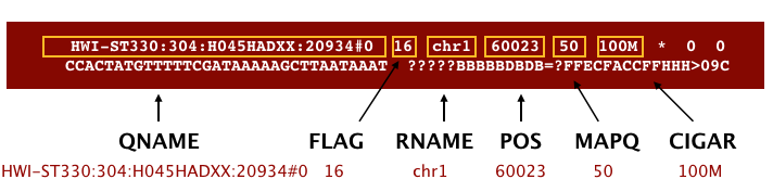
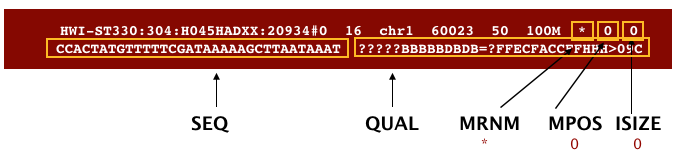
We can open and look at a SAM file because it is text, but once we start working with the BAM formatted files, we won’t be able to look at them with any text editor. So let’s go ahead and look at the formatting of a SAM file now. The SAM file begins with a header, which is optional. The header is used to describe the source of the data, the reference sequence, the method of alignment, etc., this will change depending on the aligner being used. Following the header is the alignment section. Each line that follows corresponds to alignment information for a single read. Each alignment line has 11 mandatory fields for essential mapping information and a variable number of other fields for aligner specific information. An example entry from a SAM file is displayed below with the different fields highlighted.
We will convert the SAM file to BAM format using the samtools program with the view command and tell this command that the input is in SAM format (-S) and to output BAM format (-b). We will need to use a sbatch submission script.
Name it “sam2bam.sbatch”:
#!/bin/bash
#SBATCH -p express
#SBATCH -t 1:00:00
#SBATCH --nodes=1
#SBATCH --ntasks-per-node=1
#SBATCH --mail-user=<your.email.address@univ.edu>
#SBATCH --mail-type=end
module load samtools/1.10
samtools view -S -b results/sam/SRR2584866.aligned.sam > results/bam/SRR2584866.aligned.bam
Sorting BAM files by coordinates
To manipulate the BAM files, we continue using the samtools toolset. Our next step is to sort the BAM file using the sort command from samtools. The -o flag tells the command where to write the output (only works on samtools after version 1.2).
On Pete create a submission script called bamsort.sbatch:
#!/bin/bash
#SBATCH -p express
#SBATCH -t 1:00:00
#SBATCH --nodes=1
#SBATCH --ntasks-per-node=1
#SBATCH --mail-user=<your.email.address@univ.edu>
#SBATCH --mail-type=end
module load samtools/1.10
samtools sort results/bam/SRR2584866.aligned.bam -o results/bam/SRR2584866.aligned.sorted.bam
Why do we sort these files? Because basically, DNA is linear, and putting reads in the same order as the genome, makes the rest of the mapping process run faster! But, SAM/BAM files can be sorted in multiple ways, e.g. by location of alignment on the chromosome, by read name, etc. It is important to be aware that different alignment tools will output differently sorted SAM/BAM file types, and different downstream tools require differently sorted alignment files as input.
You can use other tools in samtools to learn more about SRR2584866.aligned.bam, e.g. flagstat.
On Pete, using nano, create a submission script named flagstat.sbatch
#!/bin/bash
#SBATCH -p express
#SBATCH -t 1:00:00
#SBATCH --nodes=1
#SBATCH --ntasks-per-node=1
#SBATCH --mail-user=<your.email.address@univ.edu>
#SBATCH --mail-type=end
module load samtools/1.10
samtools flagstat results/bam/SRR2584866.aligned.sorted.bam
Save this file, and submit it. When it’s finished
the slurm-xxxxxxx.outjob output will give you the multiple statistics about your sorted bam file which you can see using the cat command:
351169 + 0 in total (QC-passed reads + QC-failed reads)
0 + 0 secondary
1169 + 0 supplementary
0 + 0 duplicates
351103 + 0 mapped (99.98% : N/A)
350000 + 0 paired in sequencing
175000 + 0 read1
175000 + 0 read2
346688 + 0 properly paired (99.05% : N/A)
349876 + 0 with itself and mate mapped
58 + 0 singletons (0.02% : N/A)
0 + 0 with mate mapped to a different chr
0 + 0 with mate mapped to a different chr (mapQ>=5)
We can’t go over all the information provided, but notice that 99.98% of the reads were mapped, and 99.05% were properly mapped as pairs. Also notice that when we saved the “unpaired” files during our quality control steps, those will show up as “singletons”, and a few of them could be used (which is better than throwing them away!).
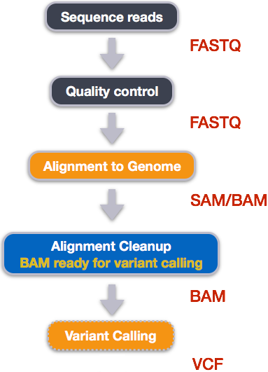
Variant calling with bcftools
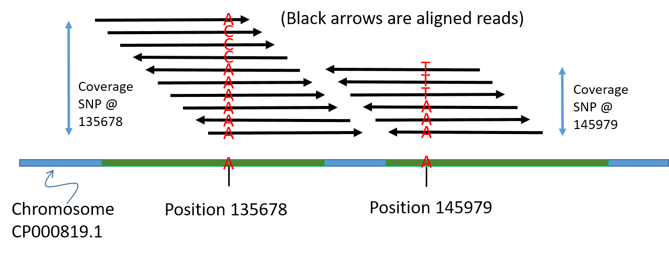
A variant call in our experiment is a conclusion that there is a nucleotide difference vs. some reference at a given position in an individual genome
or transcriptome. This type of variant is often referred to as a Single Nucleotide Polymorphism (SNP). Any variant call is usually accompanied by an estimate of
variant frequency (counts, or sometimes coverage) and some measure of confidence (can be a Phred-like score, a percentage, or even a p-value).
Similar to other steps in this workflow, there are number of tools available for
variant calling. In this workshop we will be using bcftools, but
there are a few things we need to do before actually calling the variants.
Step 1: Calculate the read coverage of positions in the genome
Coverage, is the number of times any position (a specific nucleotide) in the reference genome can be found in the sequence data. This is different than an “average” coverage of a genome, which is used in high-throughput sequencing. We can perform the first pass on variant calling by counting read coverage of any position in the genome with bcftools. We will use the command mpileup. The flag --output-type b tells samtools to generate a .bcf format output file, --output specifies where to write the output file, and --fasta-ref gives the path to the reference genome file. Note that the mpileup command expects the output file path and name to immediately follow the --output flag. The input file is the last part of the command.
On Pete, create a submission script called pileup.sbatch:
#!/bin/bash
#SBATCH -p express
#SBATCH -t 1:00:00
#SBATCH --nodes=1
#SBATCH --ntasks-per-node=1
#SBATCH --mail-user=<your.email.address@univ.edu>
#SBATCH --mail-type=end
module load bcftools
bcftools mpileup --output-type b --output results/bcf/SRR2584866_raw.bcf --fasta-ref data/ref_genome/ecoli_rel606.fasta results/bam/SRR2584866.aligned.sorted.bam
The output file should say:
[mpileup] 1 samples in 1 input files
We have now generated a file with coverage information for every base.
Here’s a visual summary of what we are identifying:
Step 2: Detect the single nucleotide polymorphisms (SNPs)
To identify SNPs we’ll use the bcftools call function. Because we are identifying SNPs in a genome, we have to pay attention to the genome “ploidy”. We specify ploidy with the flag --ploidy, which is one (1) for the haploid E. coli. The -m flag allows for multiallelic and rare-variant calling, while the -v flag tells the program to output variant sites only (not every site in the genome), and -o specifies where to write the output file. Note that bcftools call expects the path to the output file to immediately follow the -o flag. The input file is the last part of the command.
The ploidy.sbatch submission script on Pete should be:
#!/bin/bash
#SBATCH -p express
#SBATCH -t 1:00:00
#SBATCH --nodes=1
#SBATCH --ntasks-per-node=1
#SBATCH --mail-user=<your.email.address@univ.edu>
#SBATCH --mail-type=end
module load bcftools
bcftools call --ploidy 1 -m -v -o results/vcf/SRR2584866_variants.vcf results/bcf/SRR2584866_raw.bcf
For more details on the options and flags of bcftools, make sure you read the manual. After this step, we should have a lot of information about our variants, compared to the reference genome, but we need to pull out the most important information.
Step 3: Filter and report the SNP variants in variant calling format (VCF)
The VCF format is one of the most famous formats in bioinformatics! Unfortunately there are multiple versions of this format, making it difficult to work with consistently. Fortunately the bcftools package gives us a Perl script we can use to convert (or “parse”) the original .vcf file into a more standard .vcf (final) format, and output this final-formatted file.
Filter the SNPs for the final output in VCF format, using vcfutils.pl:
On Pete make a submission script named finalvcf.sbatch:
#!/bin/bash
#SBATCH -p express
#SBATCH -t 1:00:00
#SBATCH --nodes=1
#SBATCH --ntasks-per-node=1
#SBATCH --mail-user=<your.email.address@univ.edu>
#SBATCH --mail-type=end
module load bcftools
vcfutils.pl varFilter results/vcf/SRR2584866_variants.vcf  > results/vcf/SRR2584866_final_variants.vcf
The vcfutils.pl script outputs a well-formatted .vcf file we can now explore using a text editor. But this is a big and complex file.
Explore the VCF format:
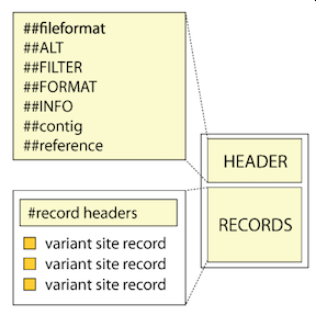 (image credit: The Broad Institute)
The basic parts of a .vcf file are the “Header”, followed by the “Records”. Both parts have important and
highly specific information. Let’s look at the file using less.
$ less -S results/vcf/SRR2584866_final_variants.vcf
You will see the header (header lines begin with ##) and describes the format, the time and date the file was
created, the version of bcftools that was used, the command line parameters used, and
lots of additional information to annotate SNPs.
##fileformat=VCFv4.2
##FILTER=<ID=PASS,Description="All filters passed">
##bcftoolsVersion=1.8+htslib-1.8
##bcftoolsCommand=mpileup --output-type b --output results/bcf/SRR2584866_raw.bcf --fasta-ref data/ref_genome/ecoli_rel606.fasta results/bam/SRR2584866.aligned.sorted.bam
##reference=file://data/ref_genome/ecoli_rel606.fasta
##contig=<ID=CP000819.1,length=4629812>
##ALT=<ID=*,Description="Represents allele(s) other than observed.">
##INFO=<ID=INDEL,Number=0,Type=Flag,Description="Indicates that the variant is an INDEL.">
##INFO=<ID=IDV,Number=1,Type=Integer,Description="Maximum number of reads supporting an indel">
##INFO=<ID=IMF,Number=1,Type=Float,Description="Maximum fraction of reads supporting an indel">
##INFO=<ID=DP,Number=1,Type=Integer,Description="Raw read depth">
##INFO=<ID=VDB,Number=1,Type=Float,Description="Variant Distance Bias for filtering splice-site artefacts in RNA-seq data (bigger is better)",Version=
##INFO=<ID=RPB,Number=1,Type=Float,Description="Mann-Whitney U test of Read Position Bias (bigger is better)">
##INFO=<ID=MQB,Number=1,Type=Float,Description="Mann-Whitney U test of Mapping Quality Bias (bigger is better)">
##INFO=<ID=BQB,Number=1,Type=Float,Description="Mann-Whitney U test of Base Quality Bias (bigger is better)">
##INFO=<ID=MQSB,Number=1,Type=Float,Description="Mann-Whitney U test of Mapping Quality vs Strand Bias (bigger is better)">
##INFO=<ID=SGB,Number=1,Type=Float,Description="Segregation based metric.">
##INFO=<ID=MQ0F,Number=1,Type=Float,Description="Fraction of MQ0 reads (smaller is better)">
##FORMAT=<ID=PL,Number=G,Type=Integer,Description="List of Phred-scaled genotype likelihoods">
##FORMAT=<ID=GT,Number=1,Type=String,Description="Genotype">
##INFO=<ID=ICB,Number=1,Type=Float,Description="Inbreeding Coefficient Binomial test (bigger is better)">
##INFO=<ID=HOB,Number=1,Type=Float,Description="Bias in the number of HOMs number (smaller is better)">
##INFO=<ID=AC,Number=A,Type=Integer,Description="Allele count in genotypes for each ALT allele, in the same order as listed">
##INFO=<ID=AN,Number=1,Type=Integer,Description="Total number of alleles in called genotypes">
##INFO=<ID=DP4,Number=4,Type=Integer,Description="Number of high-quality ref-forward , ref-reverse, alt-forward and alt-reverse bases">
##INFO=<ID=MQ,Number=1,Type=Integer,Description="Average mapping quality">
##bcftools_callVersion=1.8+htslib-1.8
##bcftools_callCommand=call --ploidy 1 -m -v -o results/bcf/SRR2584866_variants.vcf results/bcf/SRR2584866_raw.bcf; Date=Tue Oct  9 18:48:10 2018
#CHROM  POS     ID      REF     ALT     QUAL    FILTER  INFO    FORMAT  results/bam/SRR2584866.aligned.sorted.bam
CP000819.1      1521    .       C       T       207     .       DP=9;VDB=0.993024;SGB=-0.662043;MQSB=0.974597;MQ0F=0;AC=1;AN=1;DP4=0,0,4,5;MQ=60        GT:PL   1:237,0
CP000819.1      1612    .       A       G       225     .       DP=13;VDB=0.52194;SGB=-0.676189;MQSB=0.950952;MQ0F=0;AC=1;AN=1;DP4=0,0,6,5;MQ=60        GT:PL   1:255,0
It is important to know that there are variations in
.vcffiles! For example, in the header we see lots of descriptors such asID=ANandID=MQreferred to as tag-value pairs (we will learn more about metrics later) Tag-value pair descriptors and their associated metrics (e.g.AN=1andMQ=60) will vary in.vcffiles made by different softwware.
All of the header information, tag-pairs, and configuration details are followed by RECORDS: information for each of the variations observed:
#CHROM  POS  ID  REF  ALT  QUAL  FILTER  INFO  FORMAT  results/bam/SRR2584866.aligned.sorted.bam
CP000819.1  1521  .  C  T  207  .  DP=9;VDB=0.993024;SGB=-0.662043;MQSB=0.974597;MQ0F=0;AC=1;AN=1;DP4=0,0,4,5;MQ=60  GT:PL  1:237,0
CP000819.1  1612  .  A  G  225  .  DP=13;VDB=0.52194;SGB=-0.676189;MQSB=0.950952;MQ0F=0;AC=1;AN=1;DP4=0,0,6,5;MQ=60  GT:PL  1:255,0
CP000819.1  9092  .  A  G  225  .  DP=14;VDB=0.717543;SGB=-0.670168;MQSB=0.916482;MQ0F=0;AC=1;AN=1;DP4=0,0,7,3;MQ=60  GT:PL  1:255,0
CP000819.1  9972  .  T  G  214  .  DP=10;VDB=0.022095;SGB=-0.670168;MQSB=1;MQ0F=0;AC=1;AN=1;DP4=0,0,2,8;MQ=60  GT:PL  1:244,0
CP000819.1  10563  .  G  A  225  .  DP=11;VDB=0.958658;SGB=-0.670168;MQSB=0.952347;MQ0F=0;AC=1;AN=1;DP4=0,0,5,5;MQ=60  GT:PL  1:255,0
CP000819.1  22257  .  C  T  127  .  DP=5;VDB=0.0765947;SGB=-0.590765;MQSB=1;MQ0F=0;AC=1;AN=1;DP4=0,0,2,3;MQ=60  GT:PL  1:157,0
CP000819.1  38971  .  A  G  225  .  DP=14;VDB=0.872139;SGB=-0.680642;MQSB=1;MQ0F=0;AC=1;AN=1;DP4=0,0,4,8;MQ=60  GT:PL  1:255,0
CP000819.1  42306  .  A  G  225  .  DP=15;VDB=0.969686;SGB=-0.686358;MQSB=1;MQ0F=0;AC=1;AN=1;DP4=0,0,5,9;MQ=60  GT:PL  1:255,0
CP000819.1  45277  .  A  G  225  .  DP=15;VDB=0.470998;SGB=-0.680642;MQSB=0.95494;MQ0F=0;AC=1;AN=1;DP4=0,0,7,5;MQ=60  GT:PL  1:255,0
CP000819.1  56613  .  C  G  183  .  DP=12;VDB=0.879703;SGB=-0.676189;MQSB=1;MQ0F=0;AC=1;AN=1;DP4=0,0,8,3;MQ=60  GT:PL  1:213,0
CP000819.1  62118  .  A  G  225  .  DP=19;VDB=0.414981;SGB=-0.691153;MQSB=0.906029;MQ0F=0;AC=1;AN=1;DP4=0,0,8,10;MQ=59  GT:PL  1:255,0
CP000819.1  64042  .  G  A  225  .  DP=18;VDB=0.451328;SGB=-0.689466;MQSB=1;MQ0F=0;AC=1;AN=1;DP4=0,0,7,9;MQ=60  GT:PL  1:255,0
This is a lot of information, so let’s take some time to make sure we understand our output.
Here’s what the top of the RECORDS might look like if you opened it in a spreadsheet
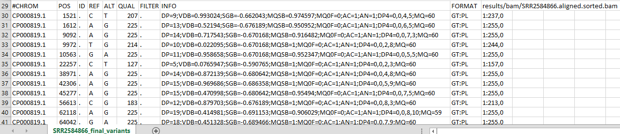
The first four columns represent the information we have about a predicted variation.
| Column | Description |
|---|---|
| CHROM | Chromosomal (or contig) where the variation occurs |
| POS | position within the chromosome (or contig) where the variation occurs |
| ID | a • is used where we did not add annotation information |
| REF | reference genotype (forward strand) |
| ALT | sample genotype (forward strand) |
| QUAL | Phred-scaled probability that the observed variant exists at this site (higher is better, maximum=99) |
| FILTER | a • means no quality filters were applied, “PASS” means a quality filter is passed, or a filter name means this variant failed that filter |
| INFO | annotations contained in the INFO field are represented as tag-value pairs (TAG=<value>) separated by semi-colon characters. TAGs are short-names for metrics. These typically summarize information from the sample. Check the header for definitions of the tag-value pairs. |
You can also find additional information on how they are calculated and how they should be interpreted in the “Variant Annotations” section of the Broad GATK Tool Documentation.
In an ideal world, the information in the QUAL column would be all we needed to filter out bad variant calls.
However, in reality we will need to continue filtering using other metrics.
The last two columns contain the GenoTypes and can be tricky to decode.
| column | definition |
|---|---|
| FORMAT | The metrics (with names derived from the header tags) of the sample-level annotations presented in a specific order and separated by colon characters. There can be several metrics (sometimes called “annotation short names”) in this column. We have two metrics: GT:PL |
| “RESULTS” (This column name varies) | lists values corresponding to every metric in the same specific order. The value follows the TAG for each locus line in the RECORDS. Values are separated by colons, but where a value (e.g. “PL”) has multiple metrics they are separated by commas (e.g. “255,0”) |
These last two columns are important for determining if the variant call is real or not. For the file in this lesson, the metrics (we requested) are presented as GT:PL which (according to the header definitions) stand for “GenoType”, and “Normalized, Phred-scaled Likelihoods for genotypes as defined in the VCF specification”. Each of these metrics will have a value, in the “RESULTS” column. The values are in the same order as the metric names, and are also separated by colon characters. These and a few other metrics and definitions are shown below:
| metric | definition |
|---|---|
| GT | The called GenoType of this sample; which for a diploid genome is encoded with a 0 for the REF allele, 1 for the first ALT allele, 2 for the second and so on. So 0/0 means homozygous reference, 0/1 (or 0/2…) means heterozygous, and 1/1 means homozygous for the alternate allele. |
| AD | the unfiltered Allele Depth, i.e. “coverage” or the number of reads that match each of the reported alleles shown as REF/ALT or sometimes REF,ALT |
| DP | the filtered sequencing DePth (Total number of reads), at the this position in the sample |
| GQ | the Genotype’s Phred-scaled quality Score (confidence) for the called genotype |
| PL | the “Normalized” Phred-scaled Likelihoods of the given genotypes. The called genotype is alwayss given a value of “0” |
Below is another example of the RECORDS part of a .vcf file borrowed from the Broad Institute website.
It has been opened in a spreadsheet, and shows some differences between our bcftools created .vcf file
and the GATK-produced .vcf file. We don’t want to be confusing, but you should remember they can be different.
Notice there are several short-name metrics under the “FORMAT” column,
each with a corresponding value under the “RESULTS” column (named NA12878 in this example). Remember that the default
metric values always put the REF value before the ALT value (REF/ALT or REF,ALT).
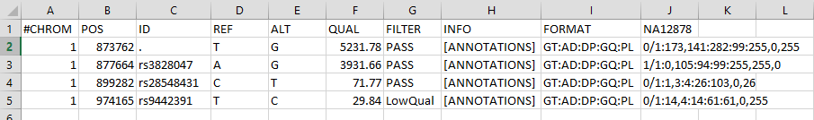 In this example, at position 873762 the metrics are:
| FORMAT | NA12878 | MEANING |
|---|---|---|
| GT | 0/1 | The called genotype is het |
| AD | 173,141 | there are 173 matches to REF, and 141 matches to ALT |
| DP | 282 | There are 282 total reads that map to this site |
| GQ | 99 | This is the highest confidence possible |
| PL | 255,0,255 | There is a 10^(-25.5) chance this is homozygous-REF, there is 10^(-0) chance this is HET, and there is 10^(-25.5) chance this is homozygous ALT |
Now you probably noticed that the PL metric has three values (255,0,255), rather than the two values
we have in our bcftools-produced .vcf file. For a detailed breakdown of the variant call at this SNP, using the Broad format,
we have created this extra page on VCF interpretation.
The Broad Institute’s VCF guide is an excellent place to learn more about VCF file format.
Do the In-class Exercise 2 by clicking on this link.
Assess the alignment (visualization) - optional step
It is often instructive to look at your data in a genome browser. Visualization will allow you to get a “feel” for the data, as well as detecting abnormalities and problems. Also, exploring the data in such a way may give you ideas for further analyses. As such, visualization tools are useful for exploratory analysis. In this lesson we will describe two different tools for visualization; a light-weight command-line based one and the Broad Institute’s Integrative Genomics Viewer (IGV) which requires software installation and transfer of files.
In order for us to visualize the alignment files, we first need to index the BAM file using samtools:
On Pete, create a submission script called samindex.sbatch:
#!/bin/bash
#SBATCH -p express
#SBATCH -t 1:00:00
#SBATCH --nodes=1
#SBATCH --ntasks-per-node=1
#SBATCH --mail-user=<your.email.address@univ.edu>
#SBATCH --mail-type=end
module load samtools
samtools index results/bam/SRR2584866.aligned.sorted.bam
You now have a file named SRR2584866.aligned.sorted.bam.bai in your /results/bam/ directory.
Viewing with IGV
IGV is a stand-alone genome browser, which has the advantage of being installed locally and providing fast access. Web-based genome browsers, like Ensembl or the UCSC browser, are slower, but provide more functionality. They not only allow for more polished and flexible visualization, but also provide easy access to a wealth of annotations and external data sources. This makes it straightforward to relate your data with information about repeat regions, known genes, epigenetic features or areas of cross-species conservation, to name just a few.
In order to use IGV, we will need to transfer some files to our local machine. We learned how to do this with scp.
Open a new tab in your LOCAL terminal window (not the one connected to a remote computer) and
create a new folder named dc_workshop on our Desktop.
Then we’ll make the directory igvfiles to store the files:
$ mkdir ~/Desktop/dc_workshop
If you get an error saying BASH cannnot make the ddirectory because the directory already exists, that is okay.
$ mkdir ~/Desktop/dc_workshop/igvfiles
Now we will transfer our files to that new directory using scp. But to make it easier, we will
combine all the files we need together into a .tar.gz file on the Pete HPC so that we only have one file to download
(and we are being good internet citizens by compressing our data and using less bandwidth).
Because compression is a slow process, we will have to write a submission script for this named gz.batch
#!/bin/bash
#SBATCH -p express
#SBATCH -t 1:00:00
#SBATCH --nodes=1
#SBATCH --ntasks-per-node=1
#SBATCH --mail-user=<your.email.address@univ.edu>
#SBATCH --mail-type=end

mkdir igvfiles
cp results/bam/SRR2584866.aligned.sorted.bam igvfiles
cp results/bam/SRR2584866.aligned.sorted.bam.bai igvfiles
cp data/ref_genome/ecoli_rel606.fasta igvfiles
cp results/vcf/SRR2584866_final_variants.vcf igvfiles
tar -czvf igvfiles.tar.gz igvfiles/*
Now we can download the igvfiles.tar.gz file from our GitBash window into our localdc_workshop directory.
scp <username>@pete.hpc.okstate.edu:/scratch/<username>/dc_workshop/igvfiles.tar.gz ~/Desktop/dc_workshop/
Then decompress our files using the matching igvfiles directory.
tar -zxvf igvfiles.tar.gz
NOTE: The tar command doesn’t create directories, which is why we had to make one for our files.
Next we need to open the IGV software. If you haven’t done so already, you can download IGV from the Broad Institute’s software page, onto your Desktop. Download the one with JAVA included. Double-click the .zip file
to unzip it, and on a Mac drag the program into your Applications folder. Windows users will find that IGV installs into
their C:Programs Files/IGV_2.11.2 folder (This will vary with newer nversions)
and also places a link to the application on their Desktop. You can copy the application link into the ~/Desktop/files_for_igv
folder you just created, or just open IGV from the Desktop
- Open IGV (double-click on the icon/link). Windows users may need to run the
.batbatch file through the Windows Command Window. - Find and load our reference genome file (
ecoli_rel606.fasta) into IGV using the “Load Genomes from File…“ option under the “Genomes” pull-down menu. - Load our BAM file (
SRR2584866.aligned.sorted.bam) using the “Load from File…“ option under the “File” pull-down menu. - Do the same with our VCF file (
SRR2584866_final_variants.vcf).
Your IGV browser might look different than the screenshot below:
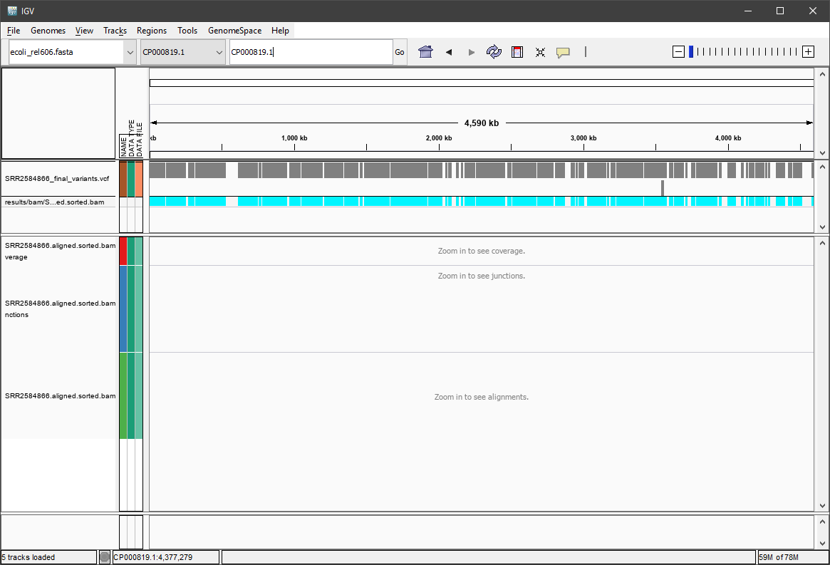
There should be two tracks: one corresponding to our BAM file and the other for our VCF file.
In the VCF track, each bar across the top of the plot shows the allele fraction for a single locus. The second bar shows the genotypes for each locus in each sample. We only have one sample called here so we only see a single line. Cyan = homozygous variant, Grey = reference. All of what we see are homozygous variants, because E. coli is a haploid organism. But with diploid organisms this row would show some heterozygous calls, and they will show up as dark-blue. Filtered entries are transparent. There might be variations in the colors for different operating systems (and you can customize them!).
We can zoom in to inspect variants you see in your filtered VCF file to become more familiar with IGV.
But first, let’s check out our hom-alt allele in the mutL gene. At the top of IGV, there is a white box
with “CP000819.1” (the chromosome number) already entered. Let’s go to position 4377265 again. Just click after
the CP000819.1 and enter a colon character then the position: :4377265 and click on “Go”.
Suddenly a lot of information is visible. It should look similar to this:
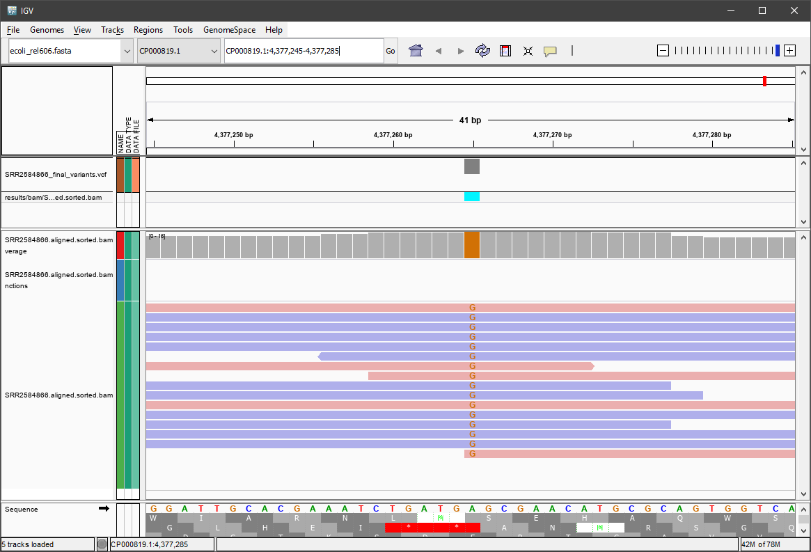
Now we can see that at position 4377265, the reference genome sequence (at the bottom) has an “A”, but all the reads (16 of them) have a “G” at that position. We also see some reads are in the forward direction, and some are in the reverse direction. We see the call is cyan colored or hom-alt. Take some time to explore this output to see how quality information corresponds to alignment information at those loci. Use this Broad Institute website and the links therein to understand how IGV colors the alignments.
Congratulations again! You have mapped over a million sequence reads to a full bacterial genome, and everything looks correct!
For a quick review of some scripting using our older shell-data directory, got to this page.
Now that we’ve run through our workflow for a single sample, we want to repeat this workflow for more
samples. However, as usual, we don’t want to type each of these individual steps again five more times. That would be very
time consuming and error-prone, and would become impossible as we gathered more and more samples. Luckily, we
already know the tools we need to use to automate this workflow and run it on as many files as we want using a
single line of code. Those tools are: wildcards, for loops, and bash scripts. We’ll use all three
in the next lesson.
Installing Software
It’s worth noting that all of the software we are using for this workshop has been pre-installed on our remote computer. This saves us a lot of time - installing software can be a time-consuming and frustrating task - however, this does mean that you won’t be able to walk out the door and start doing these analyses on your own computer. You’ll need to install the software first. Look at the setup instructions for more information on installing these software packages.
BWA Alignment options
BWA consists currently of three algorithms: BWA-backtrack, BWA-SW and BWA-MEM. The BWA-backtrack algorithm is designed only for Illumina sequence reads up to 100bp, while the other two are for sequences ranging from 70bp to 1Mbp. BWA-MEM and BWA-SW share similar features such as long-read support and split alignment, but BWA-MEM, which is the latest, is generally recommended for high-quality queries as it is faster and more accurate. We mention again that we used older software earlier to show you certain aspects of bioinformatics like being able to compare outputs, and how different software (algorithms) can produce different results. Here you can see ONE software package that has three different packages built-in!
Multi-line commands
Some of the commands we ran in this lesson are long! When typing a long command into your terminal, you can use the
\character to separate code chunks onto separate lines. This can make your code more readable.
Keypoints:
- Bioinformatics command line tools are collections of commands that can be used to carry out bioinformatics analyses.
- To use most powerful bioinformatics tools, you’ll need to use the command line.
- There are many different file formats for storing genomics data. It’s important to understand what type of information is contained in each file, and how it was derived.