OptionD Cyverse Cloud

Option D If you didn’t mean to click on OptionD, go back to the OptionA AWS page.

A Carpentries lesson, on the Cyverse cloud.

In August, 2019, The Carpentries tested a new workshop for genomics learning. This was a very different workshop. An important goal of the lesson was to show learners how to use a “Cloud” to analyze large genomic datasets. The lesson was a huge success, but started with fairly advanced learners. This was important because the later parts of the workshop used very powerful scripting in Bash and in the programming language R.

But there are many parts that beginners can learn, and we are going to explore some of those in this lesson. The first thing we need to do, is log on to a “cloud”. Fortunately, there is a free cloud infrastructure designed for scientists that we have used at OSU for 8 years. This is Cyverse. Cyverse is an NSF-funded resourcefor the research community, that is very carefully maintained and kept current with the newest methodologies. It provides training, and provides computational resources focused on genomics. Originally called “iPlant” due to it’s focus on plant genomics, Cyverse is genome-agnostic and one of the largest research facilities available for free.

Although the Carpentries workshop was hosted on the Amazon Cloud (AWS), Dr. Jason Williams put the entire workshop together on Cyverse for those who can’t pay for AWS computer time.

Cyverse: Obtain an account on Cyverse.

If you don’t already have an account on Cyverse, you should get one now. During registration, be sure to request access to the Cyverse Discovery Environment, “Atmosphere”, and Data Store (at least!). For justification, state that you are taking a course at Oklahoma State University from Dr. Peter R. Hoyt. We will be using the “Atmosphere” cloud services for this lesson.

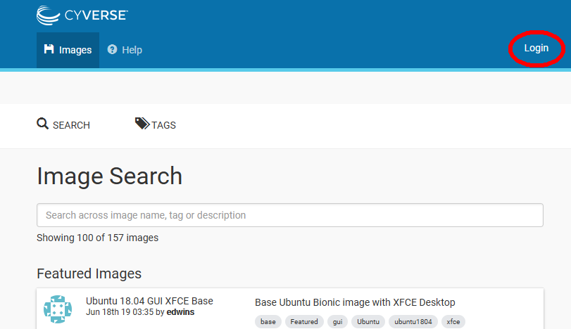
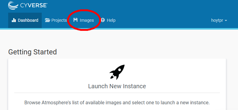
Using your web-browser, go to https://cyverse.org/atmosphere and click on the “Launch Atmosphere” button. In the next window, click on the “Login” at the upper right (circled in red below) Note that you can search for “images” in this window, but let’s login first. Enter your username and password then click on “login”. The Cyverse Atmosphere will load and the following window will give you several choices:

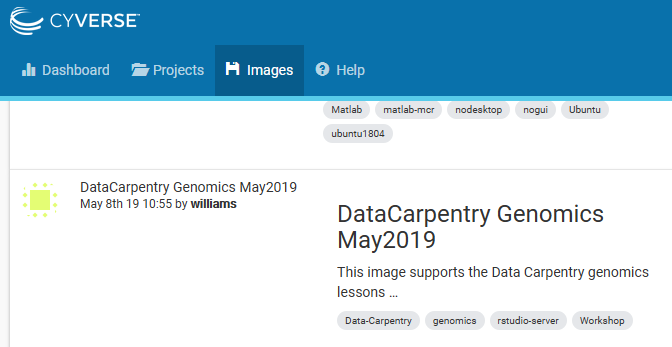
Click on the “Images tab circled in red above and you will be taken to the image search page. Here you can search for any pre-made instances. However, all you need to do is scroll down and you will soon see (in large font) the image named the “DataCarpentry Genomics May2019”

Click on the image name and you will be taken to the page describing the image, including who created it, when, and what it is used for. Specifics include software and the operating system installed as part of the image. This image also has instructions which we will use for the “Linux Lessons”. On the right side of the screen, click the blue “Launch” button!

If asked for “Resources” select “Medium 3” from the drop-down menu.

The instance should say “Launching” with a circular indicator going crazy.

Now you have to wait about 35 minutes for the image to create the instance.

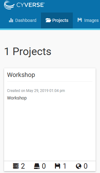
While you are waiting, return to the Atmosphere webpage, and click on the “Projects” tab to see your new “Project” called “Workshop”.

At the bottom of the “Workshop” Project window, click on the small three stacked nodes icon to see the progress of the instance.

The Instance should be “Active” under “Status” and under “Activity” should say “Deploying” with an IP Address!

The IP address is important for later, so write it down. Once the instance says “Active” with a bright green DOT, you are good to proceed.

Click on the instance name and you should see a GUI with an option to “Open web shell” near the top-right. This can be hidden from view if your browser is not set to “full-screen” mode. Click on “Open web shell”.

This will put you inside a Terminal window (In this case you are actually using the terminal from your inside your browser window!), BUT (and this is important!), you will still need to connect to the Workshop because it is a “Docker image” (we won’t be discussing these for a while, but it’s slightly similar to a virtual machine… if you are familiar with those).

To connect to the Workshop Docker image, use ssh as if it was a new computer, by entering the command ssh dcuser@127.0.0.1 -p 21 (password: data4Carp).

This command indicates that your username is “dcuser” and you want to access the computer (the Docker image of the workshop actually) at the IP address 127.0.0.1, using the port number 21.

After entering the command, you will immediately be asked for a password, which is “data4Carp”

NOTE: When we get to the R Lessons, in a NEW web browser tab, enter your Atmosphere instance IP address + “:8787” for example If your Atmosphere IP is “123.45.678” you would enter “123.45.678:8787” (user: dcuser, password: data4Carp)

Now you are inside the Genomics Workshop Cloud instance! From inside of the terminal window we start by creating a directory that we can use for the rest of the workshop/lesson. First navigate to your home directory. Use cdEnter, and confirm that you are in the correct directory using the pwd command.

$ cd
$ pwd

You should see the following as output:

/home/dcuser  

In-class Exercise

Use the mkdir command to make the following directories:

• dc_workshop
• dc_workshop/docs
• dc_workshop/data
• dc_workshop/results

Solution

$ mkdir dc_workshop
$ mkdir dc_workshop/docs
$ mkdir dc_workshop/data
$ mkdir dc_workshop/results

Use ls -R to verify that you have created these directories. The -R option for ls stands for recursive. This option causes ls to return the contents of each subdirectory within the directory iteratively.

$ ls -R dc_workshop

You should see the following output:

dc_workshop/:
data  docs  results

dc_workshop/data:

dc_workshop/docs:

dc_workshop/results: 

Organizing your files

Before beginning any analysis, it’s important to save a copy of your raw data. The raw data should never be changed. Regardless of how sure you are that you want to carry out a particular data cleaning step, there’s always the chance that you’ll change your mind later or that there will be an error in carrying out the data cleaning and you’ll need to go back a step in the process. Having a raw copy of your data that you never modify guarantees that you will always be able to start over if something goes wrong with your analysis. When starting any analysis, you can make a copy of your raw data file and do your manipulations on that file, rather than the raw version. We learned in the READINGS for todays lesson how to prevent overwriting our raw data files by setting restrictive file permissions.

NOTE: We previously used the chmod command in the Bash shell to make files executable, but this didn’t work in the Windows GitBash terminal. This is a good time to review file permissions while we are using a “real” linux environment.

We will store any results generated from our analysis in the results folder. This guarantees that we won’t confuse results file and data files in six months or two years when your future self is looking back through your files in preparation for publishing your study.

The docs folder is the place to store notes about how your analyses were carried out, any written contextual analysis of your results, and documents related to your eventual publication.

Documenting your activity on the project

When carrying out wet-lab analyses, most scientists work from a written protocol and keep a hard copy of written notes in their lab notebook. Daily notes include any things they did differently from the written protocol. This detailed record-keeping process is just as important when doing computational analyses. Luckily, it’s easier to record the steps you’ve carried out computationally than it is when working at the bench.

The history command is a convenient way to document all the commands you have used while analyzing and manipulating your project files. Let’s document the work we have done on our project so far.

View the commands that you have used so far during this session using history:

$ history

You should see that history contains all your entered shell commands. There are probably more commands than you have used for the current project. To view the last n lines of your history (where n = approximately the last few lines you think relevant) we can use tail. For our example, to view the last 7 shell commands:

$ history | tail -n 7

Using your knowledge of the shell, use the append redirect >> to create a file called dc_workshop_log_XXXX_XX_XX.sh (Use the four-digit year, two-digit month, and two digit day, e.g. dc_workshop_log_2020_10_27.sh)

You may have noticed that your history contains the history command itself. To remove this redundancy from our log, let’s use the nano text editor to fix the file:

$ nano dc_workshop_log_2020_10_27.sh

(Remember to replace the 2020_10_27 with your actual lesson or workshop date.)

From the nano screen, you can use your cursor to navigate, type, and delete line numbers, or any redundant lines.

Navigating in Nano

Although nano is useful, it can be frustrating to edit documents, as you can’t use your mouse to navigate to the part of the document you would like to edit. Here are some useful keyboard shortcuts for moving around within a text document in nano. You can find more information by typing Ctrl-G within nano.

key	action
Ctrl-Space	to move forward one word
Alt-Space	to move back one word
Ctrl-A	to move to the beginning of the current line
Ctrl-E	to move to the end of the current line
Ctrl-W	to search

Add a date line and comment to the line where you have created the directory, for example:

# 2020_10_27   
# Created sample directories for the Data Carpentry workshop  

The bash shell treats the # character as a comment character.
Any text on a line after a # character is ignored by bash when evaluating the text as code with one exeception.

Next, remove any lines of the history that are not relevant by navigating to those lines and using your delete key. Save your file and close nano.

Your file should look something like this:

# 2020_10_27
# Created sample directories for the Data Carpentry workshop

mkdir dc_workshop
mkdir dc_workshop/docs
mkdir dc_workshop/data
mkdir dc_workshop/results

If you keep this file up to date, you can use it to re-do your work on your project if something happens to your results files. To demonstrate how this works, first delete your dc_workshop directory and all of its subdirectories.

$ rm -r dc_workshop

Look at your directory contents to verify the directory is gone.

$ ls
shell_data	dc_workshop_log_2020_10_27.sh

Then run your workshop log file as a bash script. You should see the dc_workshop directory and all of its subdirectories reappear.

$ bash dc_workshop_log_2020_10_27.sh
$ ls
shell_data	dc_workshop dc_workshop_log_2020_10_27.sh

It’s important that we keep our workshop log file outside of our dc_workshop directory if we want to use it to recreate our work. It’s also important for us to keep it up to date by regularly updating with the commands that we used to generate our results files.

Congratulations! You’ve finished your introduction to using the shell for genomics projects. You now know how to navigate your file system, create, copy, move, and remove files and directories, and automate repetitive tasks using scripts and wildcards. With this solid foundation, you’re ready to move on to apply all of these new skills to carrying out more sophisticated bioinformatics analysis work. Don’t worry if everything doesn’t feel perfectly comfortable yet. We’re going to have many more opportunities for practice as we move forward on our bioinformatics journey!

References

A Quick Guide to Organizing Computational Biology Projects

Keypoints:

• “Spend the time to organize your file system when you start a new project. Your future self will thank you!”
• “Always save a write-protected copy of your raw data.”

Go Back to Data and Writing Scripts

This material is based upon work supported by the National Science Foundation under Award Numbers DBI-0735191, DBI-1265383, and DBI-1743442. URL: www.cyverse.org