
(The home directory in this lesson may vary)
Lesson based on Data Carpentry
Assessing Read Quality
Questions:
- How can I describe the quality of my data?
Objectives:
- Explain how a FASTQ file encodes per-base quality scores.
- Interpret a FastQC plot summarizing per-base quality across all reads.
- Use
forloops to automate operations on multiple files. keypoints: - Quality encodings vary across sequencing platforms.
forloops let you perform the same set of operations on multiple files with a single command.
Bioinformatics workflows
When working with high-throughput sequencing data, the raw reads you get off of the sequencer will need to pass through a number of different tools in order to generate your final desired output. The execution of this set of tools in a specified order is commonly referred to as a workflow or a pipeline.
An example of the workflow we will be using for our variant calling analysis is provided below with a brief description of each step.
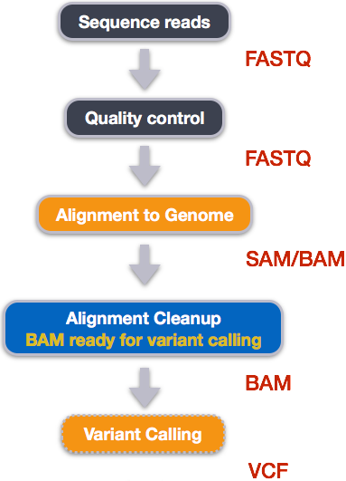
- Quality control - Assessing quality using FastQC
- Quality control - Trimming and/or filtering reads (if necessary)
- Align reads to reference genome
- Perform post-alignment clean-up
- Variant calling
These workflows in bioinformatics adopt a plug-and-play approach in that the output of one tool can be easily used as input to another tool without any extensive configuration. Having standards for data formats is what makes this feasible. Standards ensure that data is stored in a way that is generally accepted and agreed upon within the community. The tools that are used to analyze data at different stages of the workflow are therefore built under the assumption that the data will be provided in a specific format.
Starting with Data
Often times, the first step in a bioinformatics workflow is getting the data you want to work with onto a computer where you can work with it. If you have sequenced your own data, the sequencing center will usually provide you with a link that you can use to download your data. Today we will be working with publicly available sequencing data.
We are studying a population of Escherichia coli (designated Ara-3), which were propagated for more than 50,000 generations in a glucose-limited minimal medium. We will be working with three samples from this experiment, one from 5,000 generations, one from 15,000 generations, and one from 50,000 generations. The population changed substantially during the course of the experiment, and we will be exploring how with our variant calling workflow.
The data are paired-end, so we will download two files for each sample. We will use the European Nucleotide Archive to get our data. The ENA “provides a comprehensive record of the world’s nucleotide sequencing information, covering raw sequencing data, sequence assembly information and functional annotation.” The ENA also provides sequencing data in the fastq format, an important format for sequencing reads that we will be learning about today.
We are going to start in our home directory on our remote system:
To download the data, run the commands below. It will take about 10 minutes to download the files. If it seems like a file does not want to dowload, hit Cntrl-C to stop it and re-start it. Do the files one at a time so you can monitor this! First make the directory to store the files, then enter it.
mkdir -p dc_workshop/data/untrimmed_fastq/
cd dc_workshop/data/untrimmed_fastq
mkdir -p /scratch/<username>/dc_workshop/data/untrimmed_fastq/
cd /scratch/<username>/dc_workshop/data/untrimmed_fastq

curl -O ftp://ftp.sra.ebi.ac.uk/vol1/fastq/SRR258/004/SRR2589044/SRR2589044_1.fastq.gz
curl -O ftp://ftp.sra.ebi.ac.uk/vol1/fastq/SRR258/004/SRR2589044/SRR2589044_2.fastq.gz
curl -O ftp://ftp.sra.ebi.ac.uk/vol1/fastq/SRR258/003/SRR2584863/SRR2584863_1.fastq.gz
curl -O ftp://ftp.sra.ebi.ac.uk/vol1/fastq/SRR258/003/SRR2584863/SRR2584863_2.fastq.gz
curl -O ftp://ftp.sra.ebi.ac.uk/vol1/fastq/SRR258/006/SRR2584866/SRR2584866_1.fastq.gz
curl -O ftp://ftp.sra.ebi.ac.uk/vol1/fastq/SRR258/006/SRR2584866/SRR2584866_2.fastq.gz
If the curl command is going slow, stop it and use the wget command:
wget ftp://ftp.sra.ebi.ac.uk/vol1/fastq/SRR258/004/SRR2589044/SRR2589044_1.fastq.gz
wget ftp://ftp.sra.ebi.ac.uk/vol1/fastq/SRR258/004/SRR2589044/SRR2589044_2.fastq.gz
wget ftp://ftp.sra.ebi.ac.uk/vol1/fastq/SRR258/003/SRR2584863/SRR2584863_1.fastq.gz
wget ftp://ftp.sra.ebi.ac.uk/vol1/fastq/SRR258/003/SRR2584863/SRR2584863_2.fastq.gz
wget ftp://ftp.sra.ebi.ac.uk/vol1/fastq/SRR258/006/SRR2584866/SRR2584866_1.fastq.gz
wget ftp://ftp.sra.ebi.ac.uk/vol1/fastq/SRR258/006/SRR2584866/SRR2584866_2.fastq.gz
While the files are downloading, notice these sequence files are in pairs. Each pair has
the same prefix or “samplename” followed by a “1” or a “2”. These are called “paired-end”
sequence files. The file with a “1” is called the “Read1” file, and the file with the “2” is called the “Read2” file.
There must be the same number of reads in each of the paired read files. We can check this later.
The data comes in a compressed format (“gnu-zip”), which is why there is a .gz at the end of the file names.
The .gz format is a lot like the .zip format, but different, so we use the command gunzip to decompress
the file, instead of unzip. Using compressed files is always good practice. This makes it faster to
transfer, and allows it to take up less space on our computer. When the downloads are finished,
let’s unzip one of the files so that we
can look at the fastq format.
$ gunzip SRR2589044_1.fastq.gz
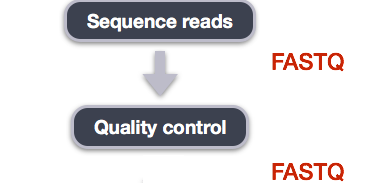
Quality Control
We will now assess the quality of the sequence reads contained in our fastq files.
Details on the FASTQ format
Although it looks complicated (and it is), we have learned the fastq format needs a little decoding. Some rules about the format include…
| Line | Description |
|---|---|
| 1 | Always begins with ‘@’ and then information about the read |
| 2 | The actual DNA sequence |
| 3 | Always begins with a ‘+’ and sometimes the same info in line 1 |
| 4 | Has a string of characters which represent the quality scores; must have same number of characters as line 2 |
We can view the first complete read in one of the files our dataset by using head to look at
the first four lines.
$ head -n 4 SRR2589044_1.fastq.gz
@SRR2584863.1 HWI-ST957:244:H73TDADXX:1:1101:4712:2181/1
TTCACATCCTGACCATTCAGTTGAGCAAAATAGTTCTTCAGTGCCTGTTTAACCGAGTCACGCAGGGGTTTTTGGGTTACCTGATCCTGAGAGTTAACGGTAGAAACGGTCAGTACGTCAGAATTTACGCGTTGTTCGAACATAGTTCTG
+
CCCFFFFFGHHHHJIJJJJIJJJIIJJJJIIIJJGFIIIJEDDFEGGJIFHHJIJJDECCGGEGIIJFHFFFACD:BBBDDACCCCAA@@CA@C>C3>@5(8&>C:9?8+89<4(:83825C(:A#########################
(NOTE if the above looks like 6 (or 8) lines, it is because Line 2 and Line 4 (and potentially Line 3) have “wrapped” around on your computer screen) Line 4 shows the quality for each nucleotide in the read. Quality is interpreted as the probability of an incorrect base call (e.g. 1 in 10) or, equivalently, the base call accuracy (e.g. 90%). To make it possible to line up each individual nucleotide with its quality score, the numerical score is converted into a character code where each individual character represents the numerical quality score for an individual nucleotide. For example, in the line above, the quality score line is:
CCCFFFFFGHHHHJIJJJJIJJJIIJJJJIIIJJGFIIIJEDDFEGGJIFHHJIJJDECCGGEGIIJFHFFFACD:BBBDDACCCCAA@@CA@C>C3>@5(8&>C:9?8+89<4(:83825C(:A#########################
The numerical value assigned to each of these characters depends on the sequencing platform that generated the reads. The sequencing machine used to generate our data uses the standard Sanger quality PHRED score encoding, using by Illumina version 1.8 onwards. Each character is assigned a quality score between 0 and 41 as shown in the chart below.
Quality character encoding: !"#$%&'()*+,-./0123456789:;<=>?@ABCDEFGHIJ
                            |         |         |         |         |
Quality score:              0........10........20........30........40
("J" = 41 = Better than 40)
Each quality score represents the probability that the corresponding nucleotide call is correct. This quality score is logarithmically based, so a quality score of 10 reflects a base call accuracy of 90%, but a quality score of 20 reflects a base call accuracy of 99%. These probability values are the results from the base calling algorithm and dependent on how much unambiguous signal was captured for the base incorporation.
Looking back at our read:
@SRR2584863.1 HWI-ST957:244:H73TDADXX:1:1101:4712:2181/1
TTCACATCCTGACCATTCAGTTGAGCAAAATAGTTCTTCAGTGCCTGTTTAACCGAGTCACGCAGGGGTTTTTGGGTTACCTGATCCTGAGAGTTAACGGTAGAAACGGTCAGTACGTCAGAATTTACGCGTTGTTCGAACATAGTTCTG
+
CCCFFFFFGHHHHJIJJJJIJJJIIJJJJIIIJJGFIIIJEDDFEGGJIFHHJIJJDECCGGEGIIJFHFFFACD:BBBDDACCCCAA@@CA@C>C3>@5(8&>C:9?8+89<4(:83825C(:A#########################
we can now see that there is a range of quality scores, but that the end
of the sequence is very poor quality (# = a quality score of 2 which is bad).
Do the In-class Exercises 1 and 2 by clicking on this link. Work on the questions yourself, before looking at the answers (take about 5 minutes).
Assessing Quality using FastQC
In real life, you won’t be assessing the quality of your reads by visually inspecting your FASTQ files. Rather, you’ll be using a software program to assess read quality and filter out poor quality reads. We’ll first use a program called FastQC to visualize the quality of our reads. Later in our workflow, we’ll use another program to filter out poor quality reads.
FastQC has a number of features which can give you a quick impression of any problems your data may have, so you can take these issues into consideration before moving forward with your analyses. Rather than looking at quality scores for each individual read, FastQC looks at quality collectively across all reads within a sample. The image below shows one FastQC-generated plot that indicates a very high quality sample:
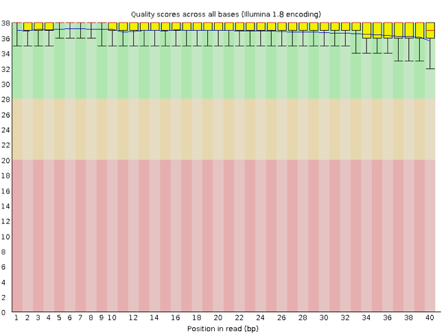
The x-axis displays the base position in the read, and the y-axis shows quality scores. In this example, the sample contains reads that are 40 bp long. This is much shorter than the reads we are working with in our workflow. For each position, there is a box-and-whisker plot showing the distribution of quality scores for all reads at that position. The horizontal red line indicates the median quality score and the yellow box shows the 2nd to 3rd quartile range. This means that 50% of reads have a quality score that falls within the range of the yellow box at that position. The whiskers show the range to the 1st and 4th quartile.
For each position in this sample, the quality values do not drop much lower than 32. This is a high quality score. The plot background is also color-coded to identify good (green), acceptable (yellow), and bad (red) quality scores.
Now let’s take a look at a quality plot on the other end of the spectrum.
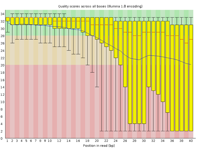
Here, we see positions within the read in which the boxes span a much wider range. Also, quality scores drop quite low into the “bad” range, particularly on the tail end of the reads. The FastQC tool produces several ther diagnostic plots to assess sample quality, in addition to the one plotted above.
Running FastQC
We will now assess the quality of the reads that we downloaded. First, make sure you’re in the untrimmed_fastq directory
$ cd /scratch/<username>/dc_workshop/data/untrimmed_fastq/
Review Exercise
How big are the files?
(Hint: Remember the options for the ls -h command to see how to show
easily understandable file sizes.)
Solution
$ ls -l -h
-rw-rw-r-- 1 dcuser dcuser 545M Jul  6 20:27 SRR2584863_1.fastq
-rw-rw-r-- 1 dcuser dcuser 183M Jul  6 20:29 SRR2584863_2.fastq.gz
-rw-rw-r-- 1 dcuser dcuser 309M Jul  6 20:34 SRR2584866_1.fastq.gz
-rw-rw-r-- 1 dcuser dcuser 296M Jul  6 20:37 SRR2584866_2.fastq.gz
-rw-rw-r-- 1 dcuser dcuser 124M Jul  6 20:22 SRR2589044_1.fastq.gz
-rw-rw-r-- 1 dcuser dcuser 128M Jul  6 20:24 SRR2589044_2.fastq.gz
There are six FASTQ files ranging from 124M (124MB) to 545M. The biggest file (SRR2584863_1.fastq) is not in compressed format
FastQC can accept multiple file names as input, and on both zipped and unzipped files, so we could use the *.fastq* wildcard to run FastQC on all of the FASTQ files in this directory. (Remember that the * wildcard character can represent “none”)
Even though fastqc runs quickly, on the Pete Computer, we’ll need to run fastqc
from a submission script.
Interactive would be great
If we were working on a cloud instance that didn’t need submission scripts we could run the files interactively. Then we would see an automatically updating output message telling you the progress of the analysis like this:
Started analysis of SRR2584863_1.fastq
Approx 5% complete for SRR2584863_1.fastq
Approx 10% complete for SRR2584863_1.fastq
Approx 15% complete for SRR2584863_1.fastq
Approx 20% complete for SRR2584863_1.fastq
Approx 25% complete for SRR2584863_1.fastq
Since running interactively is forbidden on Pete, we will create a submission script using nano. The command is:
$ nano fastqc.sbatch and when nano opens we will enter the following lines:
**From the /scratch/
#!/bin/bash
#SBATCH -p express
#SBATCH -t 1:00:00
#SBATCH --nodes=1
#SBATCH --ntasks-per-node=1
#SBATCH --mail-user=<your.email.address@okstate.edu>
#SBATCH --mail-type=end
module load fastqc/0.11.7
fastqc *.fastq*
Then save the .sbatch file and submit it:
sbatch fastqc.sbatch
In total, it should take about five minutes for FastQC to run on all
six of our FASTQ files. When it is completed, the FastQC program creates several new files within our
data/untrimmed_fastq/ directory.
$ ls
SRR2584863_1.fastq        SRR2584866_1_fastqc.html  SRR2589044_1_fastqc.html
SRR2584863_1_fastqc.html  SRR2584866_1_fastqc.zip   SRR2589044_1_fastqc.zip
SRR2584863_1_fastqc.zip   SRR2584866_1.fastq.gz     SRR2589044_1.fastq.gz
SRR2584863_2_fastqc.html  SRR2584866_2_fastqc.html  SRR2589044_2_fastqc.html
SRR2584863_2_fastqc.zip   SRR2584866_2_fastqc.zip   SRR2589044_2_fastqc.zip
SRR2584863_2.fastq.gz     SRR2584866_2.fastq.gz     SRR2589044_2.fastq.gz
For each input FASTQ file, FastQC has created a .zip file and an
.html file. The .zip file extension indicates that this is
a compressed set of multiple output files. We’ll be working
with these output files soon. The .html file is a stable webpage
displaying the summary report for each of our samples.
We want to keep our data files and our results files separate, so we
will move these
output files into a new directory within our results/ directory.
$ mkdir -p /scratch/<username>/dc_workshop/results/untrimmed_fastq_reads
$ mv *.zip /scratch/<username>/dc_workshop/results/untrimmed_fastq_reads/
$ mv *.html /scratch/<username>/dc_workshop/results/untrimmed_fastq_reads/
Now we can navigate into this results directory and do some closer inspection of our output files.
$ cd /scratch/<username>/dc_workshop/results/untrimmed_fastq_reads/
Viewing the FastQC results
If we were working on our local computers, we’d be able to display each of these HTML files as a webpage:
$ open SRR2584863_1_fastqc.html
However, if you try this on Pete or an Amazon cloud AWS instance, you’ll get an error:
Couldn't get a file descriptor referring to the console
This is because these machines don’t have any web browsers installed, so the remote computer doesn’t know how to open the file. We want to look at the webpage summary reports, so let’s transfer them to our local computers (i.e. your laptop).
To transfer a file from a remote server to our own machines, we will
use scp, which we learned yesterday in the Shell Genomics lesson.
Transferring files
First we will make a new directory on our local computer to store the HTML files we’re transferring. Let’s put it on our desktop for now. Open a new terminal (GitBash) window, or a new tab in your terminal program (if your system supports tabs, use the Cmd+t keyboard shortcut) and type:
$ mkdir Desktop/fastqc_html
Now we can transfer our HTML files to our local computer using scp.
For Pete:
$ scp <username>@pete.hpc.okstate.edu:/scratch/<username>/dc_workshop/results/untrimmed_fastq_reads/*.html ~/Desktop/fastqc_html/
As a reminder, the first part
of the command <username>@pete.hpc.okstate.edu: is
the address for your remote computer.
The second part after the : then gives the absolute path
of the files you want to transfer from your remote computer. Don’t
forget the :. We used a wildcard (*.html) to indicate that we want all of
the HTML files.
The third part of the command gives the absolute path of the location
you want to put the files. This is on your local computer and is the
directory we just created ~/Desktop/fastqc_html.
You should see a status output like this:
SRR2584863_1_fastqc.html                      100%  249KB 152.3KB/s   00:01
SRR2584863_2_fastqc.html                      100%  254KB 219.8KB/s   00:01
SRR2584866_1_fastqc.html                      100%  254KB 271.8KB/s   00:00
SRR2584866_2_fastqc.html                      100%  251KB 252.8KB/s   00:00
SRR2589044_1_fastqc.html                      100%  249KB 370.1KB/s   00:00
SRR2589044_2_fastqc.html                      100%  251KB 592.2KB/s   00:00
Now we can go to our new local directory and open the HTML files.
$ cd ~/Desktop/fastqc_html/
$ open *.html
Your computer will open each of the HTML files in your default web browser. Depending on your settings, this might be as six separate tabs in a single window or six separate browser windows.
Do the In-class Exercises 3 and 4 by clicking on this link.
Decoding the other FastQC outputs
We’ve now looked at quite a few “Per base sequence quality” FastQC graphs, but there are nine other graphs that we haven’t talked about! Below we have provided a brief overview of interpretations for each of these plots. For more information, please see the FastQC documentation here
- Per tile sequence quality: the machines that perform sequencing are divided into tiles. This plot displays patterns in base quality along these tiles. Consistently low scores are often found around the edges, but hot spots can also occur in the middle if an air bubble was introduced at some point during the run.
- Per sequence quality scores: a density plot of quality for all reads at all positions. This plot shows what quality scores are most common.
- Per base sequence content: plots the proportion of each base position over all of the reads. Typically, we expect to see each base roughly 25% of the time at each position, but this often fails at the beginning or end of the read due to quality or adapter content.
- Per sequence GC content: a density plot of average GC content in each of the reads.
- Per base N content: the percent of times that ‘N’ occurs at a position in all reads. If there is an increase at a particular position, this might indicate that something went wrong during sequencing.
- Sequence Length Distribution: the distribution of sequence lengths of all reads in the file. If the data is raw, there is often on sharp peak, however if the reads have been trimmed, there may be a distribution of shorter lengths.
- Sequence Duplication Levels: A distribution of duplicated sequences. In sequencing, we expect most reads to only occur once. If some sequences are occurring more than once, it might indicate enrichment bias (e.g. from PCR). If the samples are high coverage (or RNA-seq or amplicon), this might not be true.
- Overrepresented sequences: A list of sequences that occur more frequently than would be expected by chance.
- Adapter Content: a graph indicating where adapter sequences occur in the reads.
- K-mer Content: a graph showing any sequences which may show a positional bias within the reads.
Working with the FastQC text output
Now that we’ve looked at our HTML reports to get a feel for the data, let’s look more closely at the other output files.
Go back to the terminal program that is connected to Pete (or your cloud instance)
and make sure you’re in
our /scratch/<username>/dc_workshop/results/untrimmed_fastq_reads subdirectory.
$ cd /scratch/dc_workshop/results/untrimmed_fastq_reads/
$ ls
SRR2584863_1_fastqc.html  SRR2584866_1_fastqc.html  SRR2589044_1_fastqc.html
SRR2584863_1_fastqc.zip   SRR2584866_1_fastqc.zip   SRR2589044_1_fastqc.zip
SRR2584863_2_fastqc.html  SRR2584866_2_fastqc.html  SRR2589044_2_fastqc.html
SRR2584863_2_fastqc.zip   SRR2584866_2_fastqc.zip   SRR2589044_2_fastqc.zip
Our .zip files are compressed files and can use the program unzip
to decompress them. But the command unzip
expects to get only one zip file as input, so we cannot use wildcards
as we did with fastqc. We could go through and
unzip each file one at a time, but this is very time consuming and
error-prone. Someday you may have 500 files to unzip!
A more efficient way is to use a for loop like we learned in the Shell lessons
to iterate through all of
our .zip files. Let’s see what that looks like and then we’ll
discuss what we’re doing with each line of our loop.
$ for filename in *.zip
> do
> unzip $filename
> done
In this example, the input is six filenames (or one filename for each of our .zip files).
Each time the loop iterates, it will assign a file name to the variable filename
and run the unzip command.
The first time through the loop,
$filename is SRR2584863_1_fastqc.zip.
The interpreter runs the command unzip on SRR2584863_1_fastqc.zip.
For the second iteration, $filename becomes
SRR2584863_2_fastqc.zip. This time, the shell runs unzip on SRR2584863_2_fastqc.zip.
It then repeats this process for the four other .zip files in our directory.
When we run our for loop, you will see output that starts like this:
Archive:  SRR2589044_2_fastqc.zip
   creating: SRR2589044_2_fastqc/
   creating: SRR2589044_2_fastqc/Icons/
   creating: SRR2589044_2_fastqc/Images/
  inflating: SRR2589044_2_fastqc/Icons/fastqc_icon.png
  inflating: SRR2589044_2_fastqc/Icons/warning.png
  inflating: SRR2589044_2_fastqc/Icons/error.png
  inflating: SRR2589044_2_fastqc/Icons/tick.png
  inflating: SRR2589044_2_fastqc/summary.txt
  inflating: SRR2589044_2_fastqc/Images/per_base_quality.png
  inflating: SRR2589044_2_fastqc/Images/per_tile_quality.png
  inflating: SRR2589044_2_fastqc/Images/per_sequence_quality.png
  inflating: SRR2589044_2_fastqc/Images/per_base_sequence_content.png
  inflating: SRR2589044_2_fastqc/Images/per_sequence_gc_content.png
  inflating: SRR2589044_2_fastqc/Images/per_base_n_content.png
  inflating: SRR2589044_2_fastqc/Images/sequence_length_distribution.png
  inflating: SRR2589044_2_fastqc/Images/duplication_levels.png
  inflating: SRR2589044_2_fastqc/Images/adapter_content.png
  inflating: SRR2589044_2_fastqc/fastqc_report.html
  inflating: SRR2589044_2_fastqc/fastqc_data.txt
  inflating: SRR2589044_2_fastqc/fastqc.fo
The unzip program is decompressing the .zip files and creating
a new directory (with subdirectories) for each of our samples, to
store all of the different output that is produced by FastQC. There
are a lot of files here. The one we’re going to focus on is the
summary.txt file.
If you list the files in our directory now you will see:
SRR2584863_1_fastqc       SRR2584866_1_fastqc       SRR2589044_1_fastqc
SRR2584863_1_fastqc.html  SRR2584866_1_fastqc.html  SRR2589044_1_fastqc.html
SRR2584863_1_fastqc.zip   SRR2584866_1_fastqc.zip   SRR2589044_1_fastqc.zip
SRR2584863_2_fastqc       SRR2584866_2_fastqc       SRR2589044_2_fastqc
SRR2584863_2_fastqc.html  SRR2584866_2_fastqc.html  SRR2589044_2_fastqc.html
SRR2584863_2_fastqc.zip   SRR2584866_2_fastqc.zip   SRR2589044_2_fastqc.zip
The .html files and the uncompressed .zip files are still present,
but now we also have a new directory for each of our samples. Remember
that we can see which are directories if we use the -F flag for ls.
$ ls -F
SRR2584863_1_fastqc/      SRR2584866_1_fastqc/      SRR2589044_1_fastqc/
SRR2584863_1_fastqc.html  SRR2584866_1_fastqc.html  SRR2589044_1_fastqc.html
SRR2584863_1_fastqc.zip   SRR2584866_1_fastqc.zip   SRR2589044_1_fastqc.zip
SRR2584863_2_fastqc/      SRR2584866_2_fastqc/      SRR2589044_2_fastqc/
SRR2584863_2_fastqc.html  SRR2584866_2_fastqc.html  SRR2589044_2_fastqc.html
SRR2584863_2_fastqc.zip   SRR2584866_2_fastqc.zip   SRR2589044_2_fastqc.zip
Let’s see what files are present within one of these output directories.
$ ls -F SRR2584863_1_fastqc/
fastqc_data.txt  fastqc.fo  fastqc_report.html	Icons/	Images/  summary.txt
Use less to preview the summary.txt file for this sample.
$ less SRR2584863_1_fastqc/summary.txt
PASS    Basic Statistics        SRR2584863_1.fastq
PASS    Per base sequence quality       SRR2584863_1.fastq
PASS    Per tile sequence quality       SRR2584863_1.fastq
PASS    Per sequence quality scores     SRR2584863_1.fastq
WARN    Per base sequence content       SRR2584863_1.fastq
WARN    Per sequence GC content SRR2584863_1.fastq
PASS    Per base N content      SRR2584863_1.fastq
PASS    Sequence Length Distribution    SRR2584863_1.fastq
PASS    Sequence Duplication Levels     SRR2584863_1.fastq
PASS    Overrepresented sequences       SRR2584863_1.fastq
WARN    Adapter Content SRR2584863_1.fastq
The summary file gives us a list of tests that FastQC ran, and tells
us whether this sample passed, failed, or is borderline (WARN). Remember to quit from less you enter q.
Documenting Our Work
We can make a record of the results we obtained for all our samples
by concatenating all of our summary.txt files into a single file
using the cat command. We’ll call this full_report.txt and move
it to /scratch/<username>/dc_workshop/docs.
(You might have to make this directory)
$ cat */summary.txt > /scratch/<username>/dc_workshop/docs/full_report.txt
Other notes – Optional
Quality Encodings Vary
Although we’ve used a particular quality encoding system to demonstrate interpretation of read quality, different sequencing machines use different encoding systems. This means that, depending on which sequencer you use to generate your data, a
#may not be an indicator of a poor quality base call.This mainly relates to older Solexa/Illumina data, but it’s essential that you know which sequencing platform was used to generate your data, so that you can tell your quality control program which encoding to use. If you choose the wrong encoding, you run the risk of throwing away good reads or (even worse) not throwing away bad reads!
Same Symbols, Different Meanings
Here we see
>being used a shell prompt, whereas>is also used to redirect output. Similarly,$is used as a shell prompt, but, as we saw earlier, it is also used to ask the shell to get the value of a variable.If the shell prints
>or$then it expects you to type something, and the symbol is a prompt.If you type
>or$yourself, it is an instruction from you that the shell to redirect output or get the value of a variable.
Our next lesson is Genomics Trimming and Filtering Reads
Acknowledgments: See contributors here.