Advantages of using R

At more than 20 years old, R is fairly mature and growing in popularity. However, programming isn’t a popularity contest. Here are key advantages of analyzing data in R:

• R is open source. This means R is free - an advantage if you are at an institution where you have to pay for your own MATLAB or SAS license. Open source, is important to your colleagues in parts of the world where expensive software is inaccessible. It also means that R is actively developed by a community (see r-project.org), and there are regular updates.
• R is widely used. Ok, maybe programming is a popularity contest. Because R is used in many disciplines (not just bioinformatics), you are more likely to find help online when you need it. Chances are, almost any error message you run into, someone else has already experienced.
• R is powerful. R runs on multiple platforms (Windows/MacOS/Linux). It can work with much larger datasets than popular spreadsheet programs like Microsoft Excel, and because of its scripting capabilities is far more reproducible. Also, there are thousands of available software packages for science, particulaly statistics, data analyses, genomics and other areas of life science.

Tip: This lesson works best on the cloud

Remember, these lessons assume we are using the pre-configured virtual machine instances provided to you at a genomics workshop. Much of this work could be done on your laptop, but we use instances to simplify workshop setup requirements, and to get you familiar with using the cloud (a common requirement for working with big data). Visit the Genomics Workshop setup page for details on getting this instance running on your own, or for the info you need to do this on your own computer.

Log on to RStudio Server

Open a web browser and enter the IP address of your instance (provided by your instructors), followed by :8787. For example, if your IP address was 123.45.67.89 your URL would be

http://123.45.67.89:8787

Tip: Make sure there are no spaces before or after your URL or

your web browser may interpret it as a search query.

You should now be looking at a page that will allow you to login to the RStudio server:

Enter your user credentials and click Sign In. The credentials for the genomics Data Carpentry instances will be provided by your instructors.

You should now see the RStudio interface:

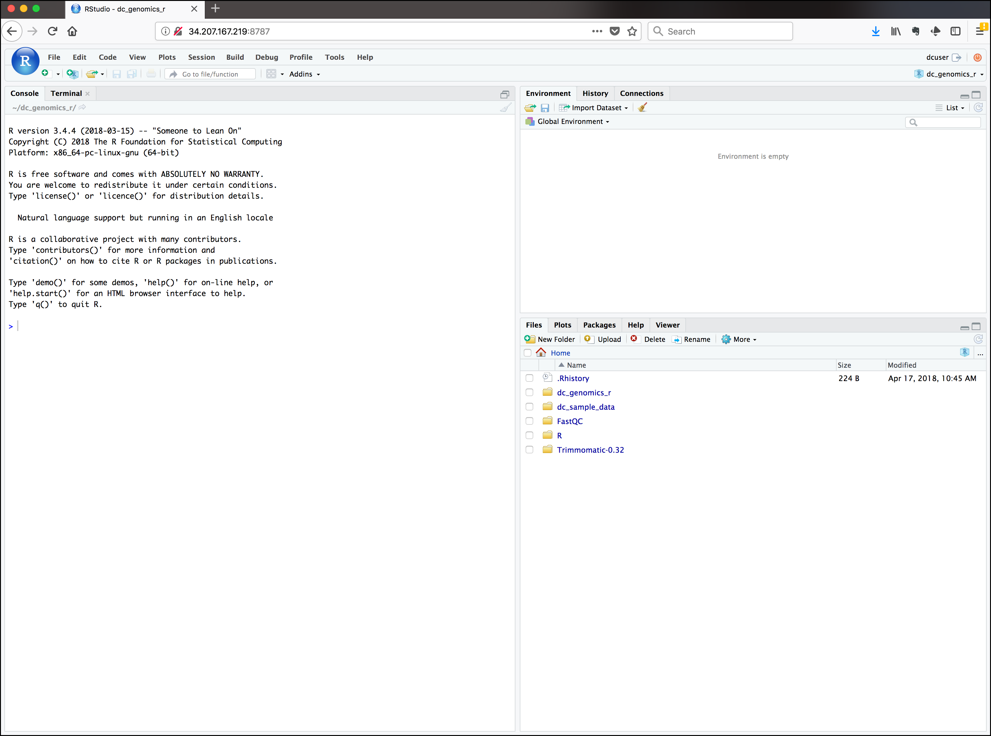
RStudio

In these lessons, we will be making use of a software called RStudio that runs R inside an IDE (an Integrated Development Environment), which operates a little like a GUI.

• Advantages:
  • The Interpreter/Console has multiple visualization panes
  • There is a Text editor that includes:
    • object-specific highlighting (easier to read)
    • provides information about problems with code (easier to understand)
    • tab key autocompletes (easy to work with)
      • Let the computer do repetitious work.
      • It makes fewer mistakes.
  • The Environment/History functions allow you to reproduce/troubleshoot something done before
  • The Project management functions keep things separate and transferable

Create an RStudio project

One of the first benefits we will take advantage of in RStudio is the Project management, by creating something called an RStudio Project. An RStudio project allows you to more easily:

• Save data, files, variables, packages, etc. related to a specific analysis project
• Restart work where you left off
• Collaborate, especially if you are using version control such as git.

1. To create a project, go to the File menu, and click New Project....

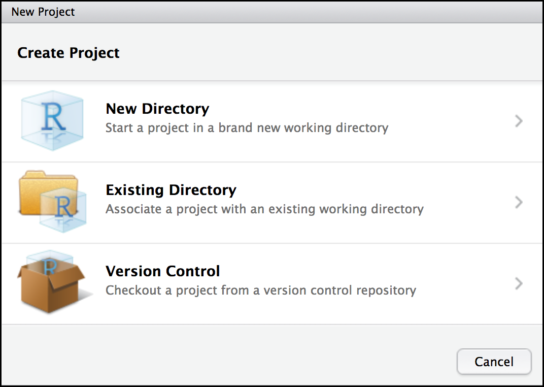
1. In the window that opens select New Directory, then New Project. For “Directory name:” enter dc_genomics_r. For “Create project as subdirectory of”, you may leave the default, which is your home directory “~”.

2. Packrat check off “Use packrat with this project” and follow any installation instructions. See the Tip below.

3. Finally click Create Project. In the “Files” tab of your output pane (more about the RStudio layout in a moment), you should see an RStudio project file, dc_genomics_r.Rproj. All RStudio projects end with the “.Rproj” file extension.

Tip: Make your project more reproducible with Packrat

One of the most wonderful and also frustrating aspects of working with R is managing packages. We will talk more about them, but packages (e.g. ggplot2) are add-ons that extend what you can do with R. Unfortunately it is very common to encounter versions of R and/or R packages that are not compatible. This makes it difficult for someone to with a different version of R or the R Packakge to run your R scripts. it’s likewise more difficult to run their scripts on your machine. Packrat is an RStudio add-on (like a package) that will associate your packages with your project so that your work is more portable and reproducible. To turn on Packrat click on the Tools menu and select Project Options.

Creating your first R script

Now that we are ready to start exploring R, we will want to keep a record of the commands we are using. To do this we can create an R script:

Click the File menu and select New File and then R Script. Before we go any further, save your script by clicking the save/disk icon that is in the bar above the first line in the script editor, or click the File menu and select save. In the “Save File” window that opens, name your file “genomics_r_basics”. The new script genomics_r_basics.R should appear under “files” in the output pane. By convention, R scripts end with the file extension .R.

Overview and customization of the RStudio layout

Although yours may be arranged differently, Here are the major windows (or panes) of the
RStudio environment:

• Source: IMPORTANT!! This pane is where you will write/view R scripts. Some outputs (such as if you view a dataset using View()) will appear as a tab here.
• Console/Terminal: This is actually where you see the execution of commands. This is the same display you would see if you were using R at the command line without RStudio. You can (but we won’t) work interactively (i.e. enter R commands here), but for the most part we will run a script (or lines in a script) in the Source pane and watch their execution and output in the Console. The “Terminal” tab gives you access to the BASH terminal (the Linux operating system, unrelated to R).
• Environment/History: Here, RStudio will show you what datasets and objects (variables) you have created and which are defined in memory. You can also see some properties of objects/datasets such as their type and dimensions. The “History” tab contains a history of the R commands you’ve executed R.
• Files/Plots/Packages/Help/Viewer: This multipurpose pane will show you the contents of directories on your computer. You can also use the “Files” tab to navigate and set the working directory. The “Plots” tab will show the output of any plots generated. In “Packages” you will see what packages are actively loaded, or you can attach installed packages. “Help” will display help files for R functions and packages. RStudio includes a Viewer pane that can be used to view local web content.

If your panes are arranged differently, you should probably go to the View menu, click on “Panes”, and then make sure “Show All Panes” and “Console on Left” are checked.

All of the panes in RStudio have configuration options. For example, you can minimize/maximize a pane, or by moving your mouse in the space between panes you can resize as needed. The most important customization options for pane layout are in the View menu. Other options such as font sizes, colors/themes, and more are in the Tools menu under Global Options.

Tip: Uploads and downloads in the cloud

In the “Files” tab you can select a file and download it from your cloud instance (click the “more” button) to your local computer. Uploads are also possible.

Yes, you are working with R!

Although we won’t be working with R at the terminal, you’ll want to use only the terminal eventually. For example, once you have written an RScript, you can run it in any Linux, Mac or Windows terminal without the need to start up RStudio.

So let’s be clear: RStudio runs R, but R is not RStudio. For more on running an R Script at the terminal see this Software Carpentry lesson.

Getting to work with R: navigating directories

Now that we have covered the more aesthetic aspects of RStudio, we can get to work using some commands. We will write, execute, and save the commands we learn in our genomics_r_basics.R script that we loaded in the Source pane. First, lets see what directory we are in. To do so, click inside the Source window, and type the following command into the script:

getwd()

To execute this command, make sure your cursor is on the same line the command is written. Then click the Run button that is just above the first line of your script in the header of the Source pane.

In the Console window, we expect to see the following output*:

[1] "/home/dcuser/dc_genomics_r"

* Notice, at the Console, you will also see the instruction you executed above the output in blue

We can predict this output when we are working on a defined system or instance such as AWS. If you are on a different machine, you might get a different directory as the default directory. For example:

[1] "C:/Users/Buddy/Desktop/R-testing/dc_genomics_r"

Since we will be learning several commands, we will want to keep some short notes or “comments” in our script to explain the purpose of the command. Putting a # before any line in an R script turns that line into a comment, which R will not try to interpret as code. To get started, edit your script to include a comment on the purpose of commands you are learning, e.g.:

# this command shows the current working directory
getwd()

For the purposes of this exercise we want you to be in the directory "/home/dcuser/R_data". What if you weren’t? You can set your home directory using the setwd() command. Enter this comment and command in your script, but don’t run this yet.

# This sets the working directory
setwd()

You may have guessed, you need to tell the setwd() command what directory you want to set as your working directory. To do so, inside of the parentheses, open a set of quotes. Inside the quotes enter a / which is the root directory for Linux. Next, use the Tab key, to take advantage of RStudio’s Tab-autocompletion method, to select home, dcuser, and dc_genomics_r directory. The path in your script should look like this:

# This sets the working directory
setwd("/home/dcuser/dc_genomics_r")

When you run this command, the console repeats the command, but gives you no output. Instead, you see the blank R prompt: >. Congratulations! Although it seems small, knowing what your working directory is and being able to set your working directory is the first step to analyzing your data.

Tip: Never use setwd()

Wait, what was the last 2 minutes about? Well, setting your working directory is something you need to do, but not as a step in your script. For example, what if your script is on a computer that has a different directory structure? The top-level path in a Unix file system is root /, but on Windows it is likely C:\. This is one of several ways you might cause a script to break because a file path is configured differently than your script anticipates. A workaround for this is to use R packages like here and file.path which allow you to specify file paths in a way that is mostly operating system independent. See Jenny Bryan’s blog post for this and other R tips.

Using functions in R, without needing to master them

A function in R (or any computing language) is a short program that takes some input and returns some output. Functions may seem like an advanced topic (and they are), but you have already used at least one function in R. getwd() is a function! The next sections will help you understand what is happening in any R script.

You have hopefully noticed a pattern - an R function has three key properties:

• Functions have a name (e.g. dir, getwd); note that functions are case sensitive!
• Following the name, functions have a pair of parentheses ()
• Inside the parentheses, a function may take 0 or more arguments

An argument may be a specific input for your function and/or may modify the function’s behavior. For example the function round() will round a number with a decimal:

 # This function will round a number to the nearest integer
round(3.14)
[1] 3

Getting help with function arguments

What if you wanted to round to one significant digit? round() can do this, but you may first need to read the help to find out how. To see the help (In R sometimes also called a “vignette”) enter a ? in front of the function name:

?round()

The “Help” tab (in the RStudio “Files/Plots/Packages/Help/Viewer” window) will show you information (often, too much information) on “Rounding of Numbers”. You will slowly learn how to read and make sense of help files. The “Usage” or “Examples” headings are often a good place to look first. If you look under the “Arguments” heading you also see what arguments can be passed to this function to modify its behavior. Alternately, you can also see the arguments for any function using the args() function:

args(round)
function (x, digits = 0) 
NULL

Using args() we see that round() takes two arguments; x, which is the number to be rounded, and a digits argument. Something to remember is that when the args() function gives you an = sign it indicates that a default (in this case 0) is already set. R will use the default value 0 unless you explicitly provide a different value. (We can ignore the NULL for now. It is returned because x doesn’t “officially” have a default value.) But it will use digits = 0 as a default. After providing x, we can explicitly set the digits parameter when we call the round() function:

round(3.14159, digits = 2)
[1] 3.14

To make things easier, R accepts what are called “positional arguments”. If you give arguments separated by commas, R assumes the arguments are in the same order as when you used args(). In the case below that means that x is 3.14159 and digits is 2 (the same as if you used digits = 2).

round(3.14159, 2)
[1] 3.14

What happens if you are using ? to get help for a function not installed on your system? Here’s an example:

?geom_point()

will return an error:

Error in .helpForCall(topicExpr, parent.frame()) :
   no methods for ‘geom_point’ and no documentation for it as a function

Use two question marks (i.e. ??geom_point()) and R will use the “Help” tab and return results from a search of all package documentation you have installed on your computer. Finally, if you think there should be a function, for example a statistical test, but you aren’t sure what it is called in R, use the “Help” tab search box.

More on finding things later

We will discuss more on where to look for the libraries and packages that contain functions you want to use. For now, be aware that two important ones are CRAN - the main repository for R, and Bioconductor - a popular repository for bioinformatics-related R packages.

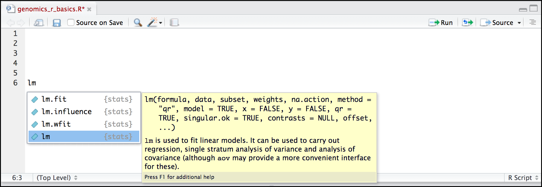
RStudio contextual help

Here is one last bonus we will mention about RStudio. It’s difficult to remember all of the arguments and definitions associated with a given function. When you start typing the name of a function and hit the Tab key, RStudio will display functions and associated help:

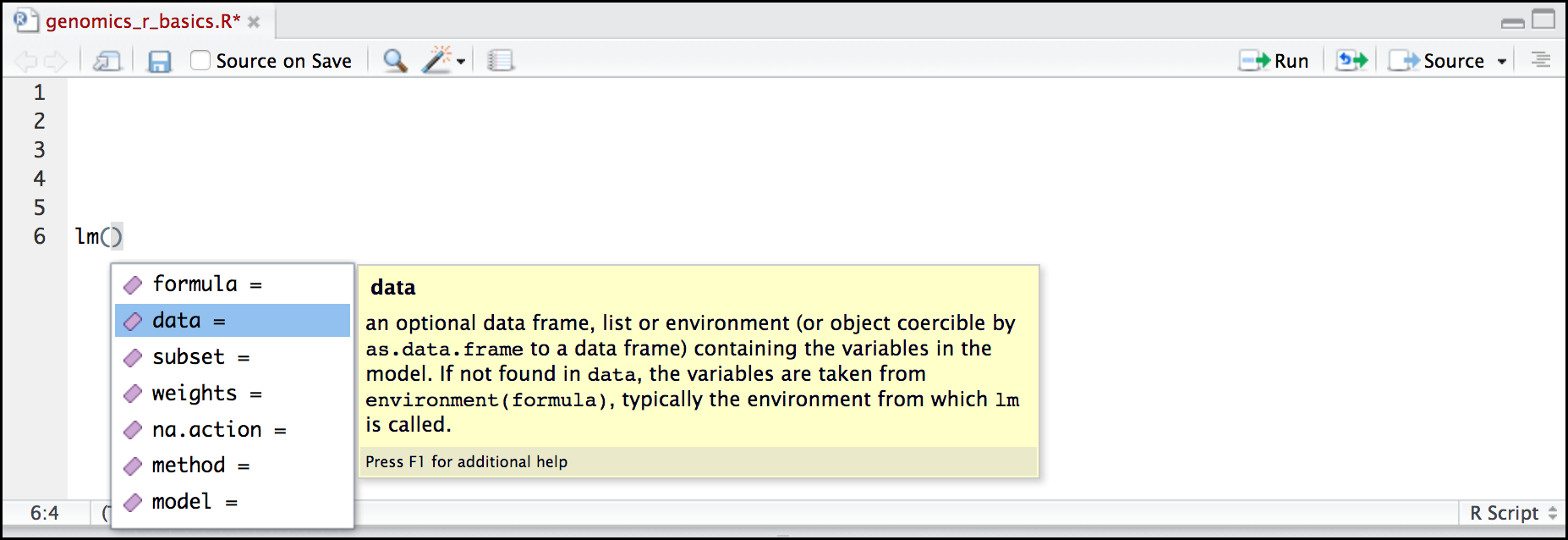
Once you type a function, hitting the Tab while the cursor is inside the parentheses will show you the function’s arguments and use the arrow keys to provide additional help for each of the arguments.

On to R Genomics

Now that we have our RStudio script running, we can begin the process of manipulating data using R. The semester is getting old, but our next lesson will be very new!