
Questions:
- How do I get started with tabular data (e.g. spreadsheets) in R?
- What are some best practices for reading data into R?
- How do I save tabular data generated in R?
Objectives:
- Understand that R uses factors to store and manipulate categorical data
- Be able to apply an arithmetic function to a data frame
- Be able to import data from Excel
- Be able to save a data frame as a delimited file
This alpha-stage lesson is an amalgam of lessons.
(use RStudio and locate combined_tidy_vcf.csv)
Working with spreadsheets (tabular data)
A substantial amount of the data we work with in genomics will be tabular data, this is data arranged in rows and columns - also known as spreadsheets. We could write a whole lesson on how to work with spreadsheets effectively (actually we did). For our purposes, we want to remind you of a few important principles before we work with our first set of example data:
1) Keep raw data separate from analyzed data
This is principle number one because if you can’t tell which files are the original raw data, you risk making some serious mistakes (e.g. drawing conclusion from data which have been manipulated in some unknown way).
2) Keep spreadsheet data Tidy
The simplest principle of Tidy data is that we have one row in our spreadsheet for each observation or sample, and one column for every variable that we measure or report on. As simple as this sounds, it’s very easily violated. Most data scientists agree that significant amounts of their time is spent tidying data for analysis (sometimes referred to as “Data Wrangling”). Read more about data organization in our lesson and in this paper.
3) Verify the data
Finally, while you don’t need to be paranoid about data, you should have a plan for how you will prepare it for analysis. Planning is a focus of this lesson. You probably already have a lot of intuition, expectations, or assumptions about your data - the range of values you expect, how many values should have been recorded, etc. But as the data get larger, our human ability to keep track will start to fail (and yes, it can fail for small data sets too). R will help you examine your data and provide greater confidence in your analysis, and its reproducibility.
Tip: Keep your raw data separate
The way R works allows you to pull data from the original file, while not actually changing the original file. This is different than (for example) working with a spreadsheet program where changing the value of the cell leaves you one “save”-click away from overwriting the original file. You have to purposely use a writing function (e.g.
write.csv()) to save data loaded into R. In that case, be sure to save the manipulated data into a new file. More on this later in the lesson.
Importing tabular data into R
There are several ways to import data into R. But for now we will
only use the tools provided in every R installation (so called “base” R) to
import a comma-delimited file containing the results of our variant calling workflow.
We will need to load the data using a function called read.csv().
Let’s start with the file combined_tidy_vcf.csv which on the AWS cloud is
located in /home/dcuser/.solutions/R_data/. Alternatively you can
find (or even read in) the file directly from [FigShare]
(https://ndownloader.figshare.com/files/14632895)
When we read in the file, we will give it an object name. Let’s call these
data variants. Remember, we are creating an object in R rather than working on the
datafile directly. This preserves our original data, while we can manipulate data
as much as we want!
The first argument to pass to our read.csv() function
is the file path for our data.
The file path must be in quotes and now is a good time
use tab autocompletion. Using tab autocompletion helps avoid typos and
errors in file paths. Use it!
## read in a CSV file and save it as 'variants'

variants <- read.csv("../r_data/combined_tidy_vcf.csv")
## silently read in CSV file from FigShare

variants <- read.csv("https://ndownloader.figshare.com/files/14632895")
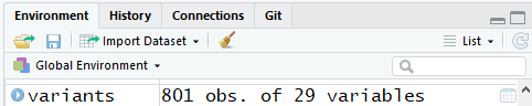
One of the first things you should notice is that in the Environment window,
you have the variants object, listed as 801 obs. (observations/rows)
of 29 variables (columns).
Summarizing and determining the structure of a data frame.
A data frame is the standard way in R to store tabular data. A data fame
could also be thought of as a collection of vectors, all of which have the same
length. We will start learning about our data frame using only two functions:
summary() and str(). These functions will
show us some summary statistics and the “structure” of the data
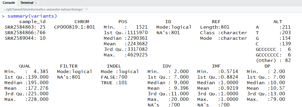
frame. Let’s start with summary():
## get summary statistics on a data frame

summary(variants)
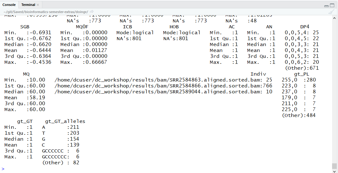
The output summary can seem a little complex at first, so here’s what happened:
First, what you see will depend on the size of your Console or Terminal window because the beginning of the summary has probably scrolled up and out of view. Scroll up to the top of the summary output. It should look something like this:
Next, by default, console only displays fields with the 6 most frequent, unique values (or categories) for each variable. Our data frame has 29 variables, so we get 29 fields that summarize the data. You can see some of these which are named “sample_id”, “CHROM”, “Pos”, etc.
We can compare the summary of our data frame with variants
in the “source” window in RStudio.
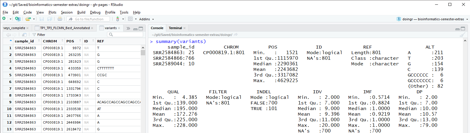
We can see these 29 variables correspond to what could be called the “column names” or the “header row”.
Notice the Pos, QUAL, and IDV variables (and several others) are
numerical data and so you get summary statistics on
the Min. and Max. values for
these columns, as well as Mean, Median, and interquartile ranges.
In contrast, many of the other variables
(e.g sample_id, CHROM, etc.) are treated as categorical data where values
are listed, along with how many times
the values are seen in the column vector.
Notice the sample_id value “SRR2584863” appeared 25
times, and, there was only one value
for CHROM which is “CP000819.1” and it appeared
in all 801 observations. Categorical data have special
treatment in R (more on this later).
Before we manipulate the data, we also need to know a little more about the
data frame structure. To do that we use the str() function:
## get the structure of a data frame

str(variants)
'data.frame':	801 obs. of  29 variables:
 $ sample_id    : Factor w/ 3 levels "SRR2584863","SRR2584866",..: 1 1 1 1 1 1 1 1 1 1 ...
 $ CHROM        : Factor w/ 1 level "CP000819.1": 1 1 1 1 1 1 1 1 1 1 ...
 $ POS          : int  9972 263235 281923 433359 473901 648692 1331794 1733343 2103887 2333538 ...
 $ ID           : logi  NA NA NA NA NA NA ...
 $ REF          : Factor w/ 59 levels "A","ACAGCCAGCCAGCCAGCCAGCCAGCCAGCCAG",..: 49 33 33 30 24 16 16 33 2 12 ...
 $ ALT          : Factor w/ 57 levels "A","AC","ACAGCCAGCCAGCCAGCCAGCCAGCCAGCCAGCCAG",..: 31 46 46 29 25 46 1 1 4 15 ...
 $ QUAL         : num  91 85 217 64 228 210 178 225 56 167 ...
 $ FILTER       : logi  NA NA NA NA NA NA ...
 $ INDEL        : logi  FALSE FALSE FALSE TRUE TRUE FALSE ...
 $ IDV          : int  NA NA NA 12 9 NA NA NA 2 7 ...
 $ IMF          : num  NA NA NA 1 0.9 ...
 $ DP           : int  4 6 10 12 10 10 8 11 3 7 ...
 $ VDB          : num  0.0257 0.0961 0.7741 0.4777 0.6595 ...
 $ RPB          : num  NA 1 NA NA NA NA NA NA NA NA ...
 $ MQB          : num  NA 1 NA NA NA NA NA NA NA NA ...
 $ BQB          : num  NA 1 NA NA NA NA NA NA NA NA ...
 $ MQSB         : num  NA NA 0.975 1 0.916 ...
 $ SGB          : num  -0.556 -0.591 -0.662 -0.676 -0.662 ...
 $ MQ0F         : num  0 0.167 0 0 0 ...
 $ ICB          : logi  NA NA NA NA NA NA ...
 $ HOB          : logi  NA NA NA NA NA NA ...
 $ AC           : int  1 1 1 1 1 1 1 1 1 1 ...
 $ AN           : int  1 1 1 1 1 1 1 1 1 1 ...
 $ DP4          : Factor w/ 217 levels "0,0,0,2","0,0,0,3",..: 3 132 73 141 176 104 61 74 133 137 ...
 $ MQ           : int  60 33 60 60 60 60 60 60 60 60 ...
 $ Indiv        : Factor w/ 3 levels "/home/dcuser/dc_workshop/results/bam/SRR2584863.aligned.sorted.bam",..: 1 1 1 1 1 1 1 1 1 1 ...
 $ gt_PL        : Factor w/ 206 levels "100,0","103,0",..: 16 10 134 198 142 127 93 142 9 80 ...
 $ gt_GT        : int  1 1 1 1 1 1 1 1 1 1 ...
 $ gt_GT_alleles: Factor w/ 57 levels "A","AC","ACAGCCAGCCAGCCAGCCAGCCAGCCAGCCAGCCAG",..: 31 46 46 29 25 46 1 1 4 15 ...
Okay, that’s a lot to take in! But you should at least be able to see
that the rows and columns of the object variants are displayed differently.
Here’s what else to notice:
- the object type
data.frameis displayed in the first row along with its dimensions, in this case 801 observations (rows) and 29 variables (columns) - Each variable has a name (e.g.
sample_id). This is followed by the object mode (i.e.int,num,logi, andFactor). - Notice that before each
variable name there is a
$- this will be important later.
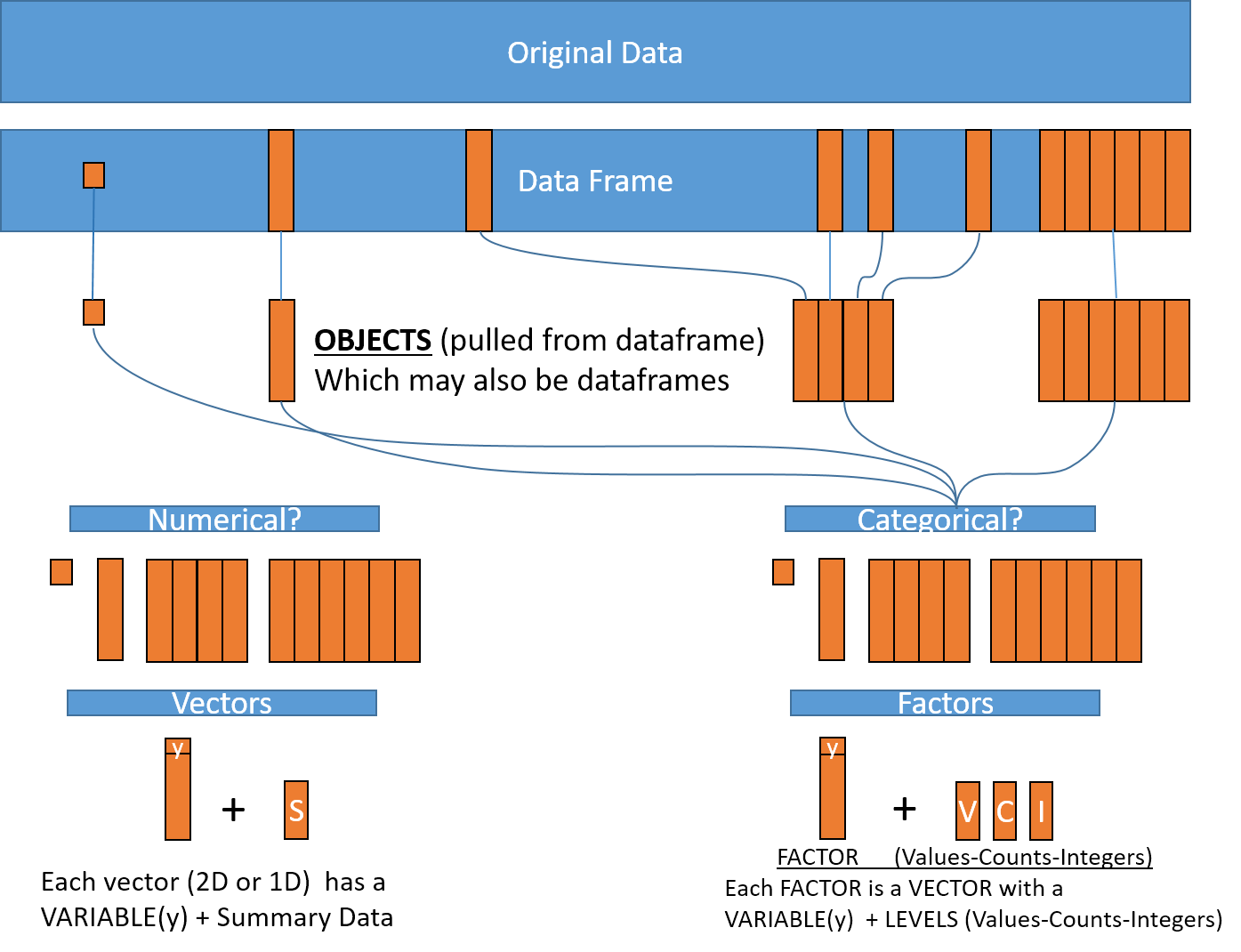
Introducing Factors
Factors are the final major data structure (mode) we will introduce in our R genomics lessons. We are only going to learn some basics about factors, but you can learn more by searching for “Factors in R”.
Factors can be thought of as vectors which are specialized for categorical data. Because R is specialized for statistics, it makes sense to have a way to deal with categorical data as if they were continuous (e.g. numerical) data.
Sometimes you may want to have data treated as a factor, but not always! Since some of the data in our data frame are already identified as factors, lets see how factors work!
First, we’ll extract one of the (non-numerical) columns of our data frame
to a new object, so that we don’t end up modifying the variants
object by mistake. Here’s where we use the $. In R, the dollar
sign ($) has a special meaning. It means that whatever comes directly
after it is a column in a data frame:
## extract the "REF" column to a new object

REF <- variants$REF
The “REF” column had a mode of “chr” or “character”. Let’s look at the first few items in our object using head():
head(REF)
[1] T        G        G        CTTTTTTT CCGC     C
59 Levels: A ACAGCCAGCCAGCCAGCCAGCCAGCCAGCCAG ... TGGGGGGG
What we get back are two lines. The first line represents a shortened form of all the items in our object (think: everything in the column). The second line is something called “Levels”. Levels are the unique categories of a factor (think: every unique value in the column). By default, R will organize the levels in a factor in alphabetical order. So the first level in this factor is “A”.
Lets look at the contents of a factor in a slightly different way using str():
str(REF)
 Factor w/ 59 levels "A","ACAGCCAGCCAGCCAGCCAGCCAGCCAGCCAG",..: 49 33 33 30 24 16 16 33 2 12 ...
The first thing we see with the str() function is that this factor
has 59 levels. The the values (or categories) of those levels are displayed
in alphabetic order. Those are the unique levels again. The second part of
str() tells us the integer assigned to each level using the
original order of “REF”.
Say that again??
For the sake of efficiency, R stores the content of a factor as a vector with integers. Once the contents in the object are arranged in alphabetical order, all identical values are merged creating a “level”. Each level has a unique value (and there are 59 of them in “REF”) which is assigned an integer.
The head() function told us the first value in our “REF” object
is “T”, but the second part of the str() output tells us that
“T” in alphabetical order happens to be at the 49th level
of our factor. According to head() the next two values
from the top are both “G”s, and str() tells us that
“G” is the 33rd level of our factor.
How is this more efficient?
Think of a column with 10,000 values! If 9,997 of the values are “ABC” and 3 of the values are “XYZ”, a computer might store the information in two “levels” as (9997ABC1, 3XYZ2) rather than having to keep all 10,000 values in memory.
Even if the computer had to remember the 3 “XYZ” values were originally at positions 384, 1768, and 7899 in the column, all the information for the column could be stored something like:
(9998ABC1, 2XYZ2[384,1768,7899]).That’s 32 characters instead of 30,000 characters and includes the levels/values (ABC, XYZ) the counts (9998, 2) and the integers (1, 2) with positional information!!!!
When we call a function like
str(), R uses stored vectors to re-display the object values.
Maybe a chart will help?
Plotting and ordering factors
One of the most common uses for factors will be when you plot categorical values. For example, suppose we want to know how many of our variants had each possible nucleotide (or nucleotide combination) in the reference genome? We could generate a plot:
plot(REF)
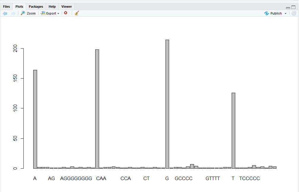
This was easy, but isn’t a particularly pretty example of a plot. We’ll be learning much more about creating nice, publication-quality graphics later in this lesson.
One more thing. When you are referring to, or requesting from, a two-dimensional dataframe
it’s not hard to understand that you’ll need to use the row, and the column, of
whatever you refer to. But you must always refer to “ROW” first, and then “COLUMN”.
Example:
“dataObject[2,4]” means “give me whatever is in the 2nd row and 4th column
of the data frame called ‘dataObject’”
To remember this convention, try thinking of “RC Cola”. In the brand’s name, “RC” stands for “Royal Crown”… but we can pretend it stands for “Row Column”.
Data frame bonus material: math, sorting, renaming
Here are a few operations that don’t need much explanation, but which are good to know.
There are lots of arithmetic functions you may want to apply to your data frame, covering those would be a course in itself (there is some starting material here). Our lessons will cover some additional summary statistical functions in a subsequent lesson, but overall we will focus on data cleaning and visualization.
You can use functions like mean(), min(), max() on an
individual column. Let’s look at the “DP” or filtered depth. This value shows the number of filtered
reads that support each of the reported variants.
max(variants$DP)
You can sort a data frame using the order() function:
sorted_by_DP <- variants[order(variants$DP), ]
head(sorted_by_DP$DP)
Exercise
The
order()function lists values in increasing order by default. Look at the documentation for this function and changesorted_by_DPto start with variants with the largest filtered depth (“DP”).Solution
sorted_by_DP <- variants[order(variants$DP, decreasing = TRUE), ]
head(sorted_by_DP$DP)
You can rename columns:
colnames(variants)[colnames(variants) == "sample_id"] <- "strain"

# check the column name (hint names are returned as a vector)
colnames(variants)
Saving your data frame to a file
We can save data to a file. We will save our SRR2584863_variants object
to a .csv file using the write.csv() function:
write.csv(SRR2584863_variants, file = "../data/SRR2584863_variants.csv")
The write.csv() function has some additional arguments listed in the help, but
at a minimum you need to tell it what data frame to write to file, and give a
path to a file name in quotes (if you only provide a file name, the file will
be written in the current working directory).
Importing data from Excel
Excel is one of the most common formats, so we need to discuss how to make these files play nicely with R. The simplest way to import data from Excel is to save your Excel file in .csv format*. You can then import into R right away. Sometimes you may not be able to do this (imagine you have data in 300 Excel files, are you going to open and export all of them?).
One common R package (a set of code with features you can download and add to your R installation) is the readxl package which can open and import Excel files. Rather than addressing package installation this second (we’ll discuss this soon!), we can take advantage of RStudio’s import feature which integrates this package. (Note: this feature is available only in the latest versions of RStudio such as is installed on our cloud instance).
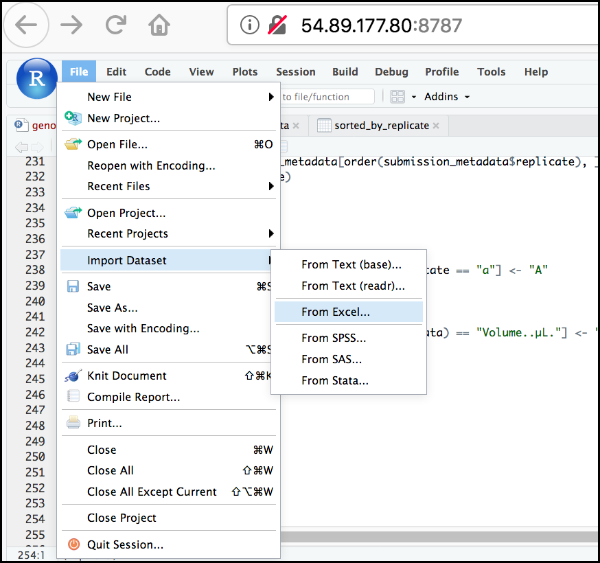
First, in the RStudio menu go to File, select Import Dataset, and choose From Excel… (notice there are several other options you can explore). If asked to install or update files, go ahead and say yes, it will only take a few seconds.
Next, under File/Url: click the Browse button and navigate to the Ecoli_metadata.xlsx file located at /home/dcuser/dc_sample_data/R.
(On your system it could be in /data/Ecoli_metadata.xlsx)
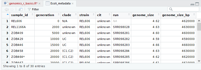
You should now see a preview of the data to be imported:
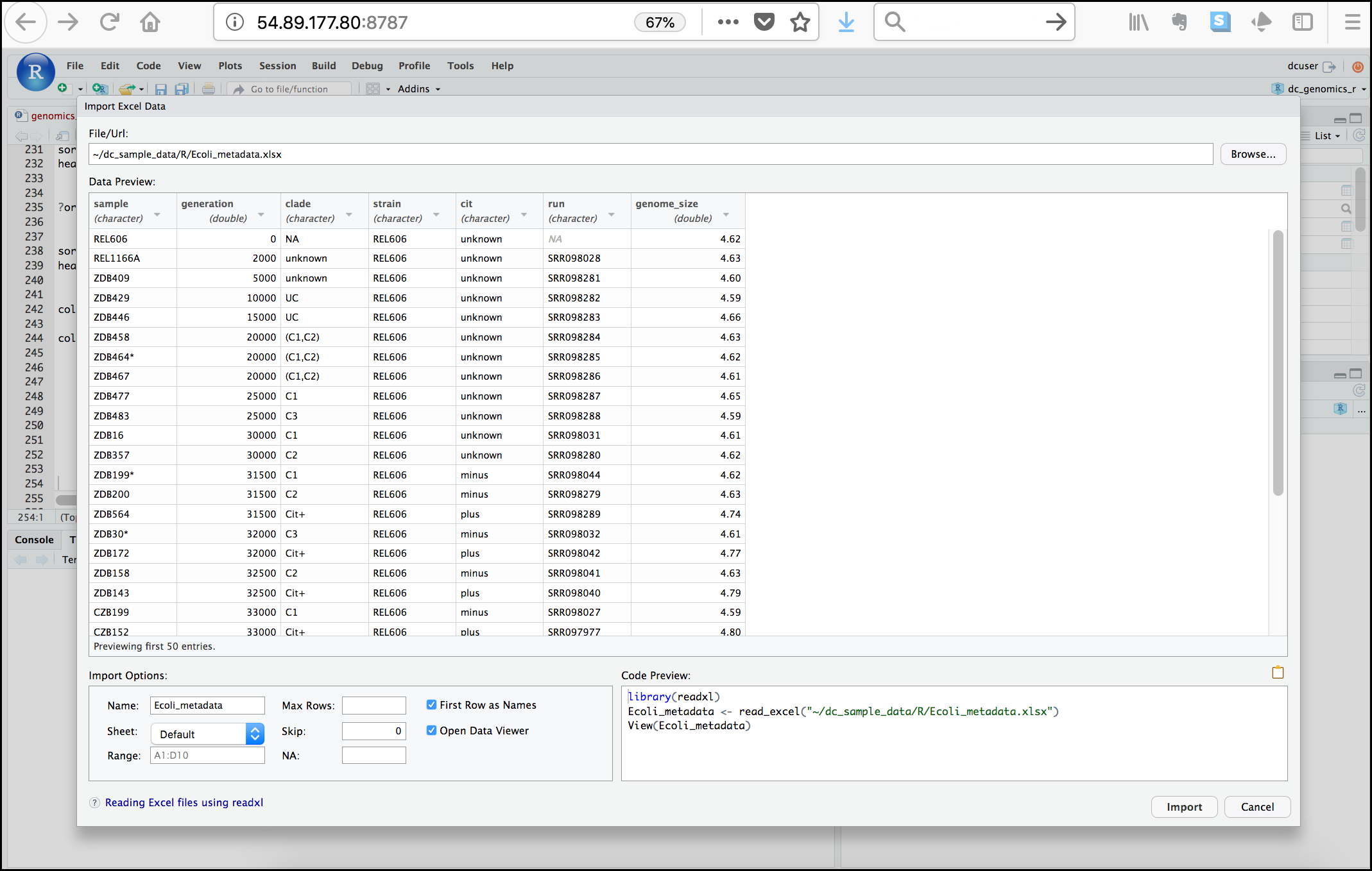
Notice that you have the option to change the data type of each variable by clicking arrow (drop-down menu) next to each column title. Under Import Options you may also rename the data, choose a different sheet to import, and choose how you will handle headers and skipped rows. Under Code Preview you can see the code that will be used to import this file. We could have written this code and imported the Excel file without the RStudio import function, but now you can choose your preference.
In this exercise, we will leave the title of the data frame as Ecoli_metadata, and there are no other options we need to adjust. Click the Import button to import the data. RStudio will show new DATA under the Environment tab of the Data window, and a new tab showing the imported data will show in the “Source” window. Change back to the “genomics_r_basics.R” script window of the Source window.
Finally, let’s check the first few lines of the Ecoli_metadata data
frame:
## read the file so the rest of the episode works, but don't show the code
Ecoli_metadata <-  readxl::read_xlsx("../data/Ecoli_metadata.xlsx")
head(Ecoli_metadata)
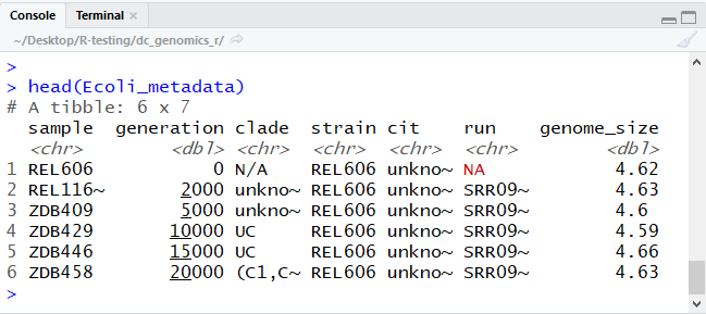
The type of this object is ‘tibble’, a type of data
frame we will talk more about in the ‘dplyr’ section. If you needed
a true R data frame you could coerce with as.data.frame().
Do Exercise Genomics-rstudio-R-4
Exercise: Putting it all together - data frames
Using the
Ecoli_metadatadata frame created above, answer the following questionsA) What are the dimensions (# rows, # columns) of the data frame?
B) What are categories are there in the
citcolumn? hint: treat column as factorC) How many of each of the
citcategories are there?D) What is the genome size for the 7th observation in this data set?
E) What is the median value of the variable
genome_sizeF) Rename the column
sampletosample_idG) Create a new column (name genome_size_bp) and set it equal to the genome_size multiplied by 1,000,000
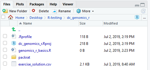
H) Save the edited Ecoli_metadata data frame as “exercise_solution.csv” in your current working directory.
When you are done, your RStudio windows should look like this:
Keypoints:
- It is easy to import data into R from tabular formats including Excel. However, you still need to check that R has imported and interpreted your data correctly
- There are best practices for organizing your data (keeping it tidy) and R is great for this
- Base R has many useful functions for manipulating your data, but all of R’s capabilities are greatly enhanced by software packages developed by the community