Objectives
- Understand how R may coerce data into different modes
- Be able to coerce the class of an object (including variables in a data frame)
- Understand that lists can hold data of more than one mode and can be indexed and coerced to different modes
Coercing values in data frames
What is coercion?
Changing the mode of an object intentionally.
Tip: coercion isn’t limited to data frames
While we are going to address coercion in the context of data frames most of these methods apply to other data structures, such as vectors
Sometimes, it is possible that R will misinterpret the type of data represented in a data frame, or store that data in a mode which prevents you from operating on the data the way you wish. For example, a long list of gene names isn’t usually thought of as a categorical variable, the way that your experimental condition (e.g. control, treatment) might be. More importantly, some R packages you use to analyze your data may expect characters as input, not factors. At other times (such as plotting or some statistical analyses) a factor may be more appropriate. Ultimately, you should know how to change the mode of an object.
First, its very important to recognize that coercion happens in R all the time. This can be a good thing when R gets it right, or a bad thing when the result is not what you expect. Consider:
snp_chromosomes <- c('3', '11', 'X', '6')
typeof(snp_chromosomes)
[1] "character"
Although there are several numbers in our vector, they are all in quotes, so we have explicitly told R to consider them as characters. However, even if we removed the quotes from the numbers, R would coerce everything into a character:
snp_chromosomes_2 <- c(3, 11, 'X', 6)
typeof(snp_chromosomes_2)
[1] "character"
snp_chromosomes_2
[1] "3"  "11" "X"  "6"
We can use the as. functions to explicitly coerce values from one form into
another. Consider the following vector of characters, which all happen to be
valid numbers:
snp_positions_2 <- c("8762685", "66560624", "67545785", "154039662")
typeof(snp_positions_2)
[1] "character"
Now we can coerce snp_positions_2 into a numeric type using as.numeric():
snp_positions_2 <- as.numeric(snp_positions_2)
typeof(snp_positions_2)
[1] "double"
snp_positions_2
[1]   8762685  66560624  67545785 154039662
Sometimes coercion is straight forward, but what would happen if we tried
using as.numeric() on snp_chromosomes_2
snp_chromosomes_2
[1] "3"  "11" "X"  "6"
snp_chromosomes_2 <- as.numeric(snp_chromosomes_2)
Warning message:
NAs introduced by coercion
If we check, we will see that an NA value (R’s default value for missing
data) has been introduced. Basically there is NO WAY to coerce a “X”
into a numeric. So now when we look at snp_chrmosomes we see
“X” has been replaced with an ‘NA’.
snp_chromosomes_2
[1]  3 11 **NA**  6
Trouble can really start when we try to coerce a factor. For example, when we
try to coerce the sample_id column in our original data frame into a
numeric mode.
Look at the result:
as.numeric(variants$sample_id)
  [1] 1 1 1 1 1 1 1 1 1 1 1 1 1 1 1 1 1 1 1 1 1 1 1 1 1 2 2 2 2 2 2 2
 [33] 2 2 2 2 2 2 2 2 2 2 2 2 2 2 2 2 2 2 2 2 2 2 2 2 2 2 2 2 2 2 2 2
 [65] 2 2 2 2 2 2 2 2 2 2 2 2 2 2 2 2 2 2 2 2 2 2 2 2 2 2 2 2 2 2 2 2
 [97] 2 2 2 2 2 2 2 2 2 2 2 2 2 2 2 2 2 2 2 2 2 2 2 2 2 2 2 2 2 2 2 2
[129] 2 2 2 2 2 2 2 2 2 2 2 2 2 2 2 2 2 2 2 2 2 2 2 2 2 2 2 2 2 2 2 2
[161] 2 2 2 2 2 2 2 2 2 2 2 2 2 2 2 2 2 2 2 2 2 2 2 2 2 2 2 2 2 2 2 2
[193] 2 2 2 2 2 2 2 2 2 2 2 2 2 2 2 2 2 2 2 2 2 2 2 2 2 2 2 2 2 2 2 2
[225] 2 2 2 2 2 2 2 2 2 2 2 2 2 2 2 2 2 2 2 2 2 2 2 2 2 2 2 2 2 2 2 2
[257] 2 2 2 2 2 2 2 2 2 2 2 2 2 2 2 2 2 2 2 2 2 2 2 2 2 2 2 2 2 2 2 2
[289] 2 2 2 2 2 2 2 2 2 2 2 2 2 2 2 2 2 2 2 2 2 2 2 2 2 2 2 2 2 2 2 2
[321] 2 2 2 2 2 2 2 2 2 2 2 2 2 2 2 2 2 2 2 2 2 2 2 2 2 2 2 2 2 2 2 2
[353] 2 2 2 2 2 2 2 2 2 2 2 2 2 2 2 2 2 2 2 2 2 2 2 2 2 2 2 2 2 2 2 2
[385] 2 2 2 2 2 2 2 2 2 2 2 2 2 2 2 2 2 2 2 2 2 2 2 2 2 2 2 2 2 2 2 2
[417] 2 2 2 2 2 2 2 2 2 2 2 2 2 2 2 2 2 2 2 2 2 2 2 2 2 2 2 2 2 2 2 2
[449] 2 2 2 2 2 2 2 2 2 2 2 2 2 2 2 2 2 2 2 2 2 2 2 2 2 2 2 2 2 2 2 2
[481] 2 2 2 2 2 2 2 2 2 2 2 2 2 2 2 2 2 2 2 2 2 2 2 2 2 2 2 2 2 2 2 2
[513] 2 2 2 2 2 2 2 2 2 2 2 2 2 2 2 2 2 2 2 2 2 2 2 2 2 2 2 2 2 2 2 2
[545] 2 2 2 2 2 2 2 2 2 2 2 2 2 2 2 2 2 2 2 2 2 2 2 2 2 2 2 2 2 2 2 2
[577] 2 2 2 2 2 2 2 2 2 2 2 2 2 2 2 2 2 2 2 2 2 2 2 2 2 2 2 2 2 2 2 2
[609] 2 2 2 2 2 2 2 2 2 2 2 2 2 2 2 2 2 2 2 2 2 2 2 2 2 2 2 2 2 2 2 2
[641] 2 2 2 2 2 2 2 2 2 2 2 2 2 2 2 2 2 2 2 2 2 2 2 2 2 2 2 2 2 2 2 2
[673] 2 2 2 2 2 2 2 2 2 2 2 2 2 2 2 2 2 2 2 2 2 2 2 2 2 2 2 2 2 2 2 2
[705] 2 2 2 2 2 2 2 2 2 2 2 2 2 2 2 2 2 2 2 2 2 2 2 2 2 2 2 2 2 2 2 2
[737] 2 2 2 2 2 2 2 2 2 2 2 2 2 2 2 2 2 2 2 2 2 2 2 2 2 2 2 2 2 2 2 2
[769] 2 2 2 2 2 2 2 2 2 2 2 2 2 2 2 2 2 2 2 2 2 2 2 3 3 3 3 3 3 3 3 3
[801] 3
Strangely, it almost works! Instead of giving an error message, R returns numeric values. BUT these numeric values are the integers assigned to the levels in this factor. This kind of behavior can lead to hard-to-find bugs, for example when we expect to have numbers in a factor, and we get numbers from a coercion. But they the intergers, not the values. If we don’t look carefully, we may not notice a problem.
One more note about coercion: If you need to coerce an entire column you can overwrite it using an expression like this one:
# make the 'REF' column a character type column

variants$REF <- as.character(variants$REF)

# check the type of the column
typeof(variants$REF)
[1] "character"
–>
Coercion take home messages
- When you explicitly coerce one data type into another (this is known as explicit coercion), be careful to check the result. Ideally, you should try to avoid steps in your analysis that force you to coerce (if possible).
- R will sometimes coerce without you asking for it. This is called (appropriately) implicit coercion. For example when we tried to create a vector that had multiple data types, R chose one type through implicit coercion.
- Check the structure (
str()) of your data frames after coercion (or maybe always) before working with them!Using StringsAsFactors = FALSE
One way to avoid needless coercion when importing a data frame using any one of the
read.table()functions (e.g.read.csv()) is to use the argumentStringsAsFactorsset to FALSE (i.e.StringsAsFactors = FALSE). By default, this argument is TRUE. Setting it to FALSE will treat any non-numeric column as “character” type. Some programmers set this as the default in R.Example
Read in read.csv again as variantsSTR using StringsAsFactors = FALSE
variantsStr <- read.csv("https://ndownloader.figshare.com/files/14632895", stringsAsFactors = FALSE)
str(variantsStr)
'data.frame':	801 obs. of  29 variables:
 $ sample_id    : chr  "SRR2584863" "SRR2584863" "SRR2584863" "SRR2584863" ...
 $ CHROM        : chr  "CP000819.1" "CP000819.1" "CP000819.1" "CP000819.1" ...
 $ POS          : int  9972 263235 281923 433359 473901 648692 1331794 1733343 2103887 2333538 ...
 $ ID           : logi  NA NA NA NA NA NA ...
 $ REF          : chr  "T" "G" "G" "CTTTTTTT" ...
 $ ALT          : chr  "G" "T" "T" "CTTTTTTTT" ...
 $ QUAL         : num  91 85 217 64 228 210 178 225 56 167 ...
 $ FILTER       : logi  NA NA NA NA NA NA ...
 $ INDEL        : logi  FALSE FALSE FALSE TRUE TRUE FALSE ...
 $ IDV          : int  NA NA NA 12 9 NA NA NA 2 7 ...
 $ IMF          : num  NA NA NA 1 0.9 ...
 $ DP           : int  4 6 10 12 10 10 8 11 3 7 ...
 $ VDB          : num  0.0257 0.0961 0.7741 0.4777 0.6595 ...
 $ RPB          : num  NA 1 NA NA NA NA NA NA NA NA ...
 $ MQB          : num  NA 1 NA NA NA NA NA NA NA NA ...
 $ BQB          : num  NA 1 NA NA NA NA NA NA NA NA ...
 $ MQSB         : num  NA NA 0.975 1 0.916 ...
 $ SGB          : num  -0.556 -0.591 -0.662 -0.676 -0.662 ...
 $ MQ0F         : num  0 0.167 0 0 0 ...
 $ ICB          : logi  NA NA NA NA NA NA ...
 $ HOB          : logi  NA NA NA NA NA NA ...
 $ AC           : int  1 1 1 1 1 1 1 1 1 1 ...
 $ AN           : int  1 1 1 1 1 1 1 1 1 1 ...
 $ DP4          : chr  "0,0,0,4" "0,1,0,5" "0,0,4,5" "0,1,3,8" ...
 $ MQ           : int  60 33 60 60 60 60 60 60 60 60 ...
 $ Indiv        : chr  "/home/dcuser/dc_workshop/results/bam/SRR2584863.aligned.sorted.bam" "/home/dcuser/dc_workshop/results/bam/SRR2584863.aligned.sorted.bam" "/home/dcuser/dc_workshop/results/bam/SRR2584863.aligned.sorted.bam" "/home/dcuser/dc_workshop/results/bam/SRR2584863.aligned.sorted.bam" ...
 $ gt_PL        : chr  "121,0" "112,0" "247,0" "91,0" ...
 $ gt_GT        : int  1 1 1 1 1 1 1 1 1 1 ...
 $ gt_GT_alleles: chr  "G" "T" "T" "CTTTTTTTT" ...
Notice that there are no “factor” coulmns in our data frame. Most coulmns that showed up as “factors” mode in the dataframe variants are now chr or “character” mode in variantsStr You can look at the vector for variable “ALT” and see they don’t have assigned “levels”).
> summary (variantsStr$ALT)
   Length     Class      Mode
      801 character character
> summary (variants$ALT)
                                                       A
                                                     211
                                                      AC
                                                       2
                    ACAGCCAGCCAGCCAGCCAGCCAGCCAGCCAGCCAG
                                                       1
(etc.)
The read.csv() documentation, also shows you how to
explicitly set your columns to a specific type using the colClasses argument.
Other R packages (such as the Tidyverse “readr”) don’t have this
particular coercion issue,
but many packages will try to guess a data type.
Check your structures!
Bonus Section
(Material based on http://monashbioinformaticsplatform.github.io/2015-09-28-rbioinformatics-intro-r/01-supp-factors.html)
Working with coercion and factors
Coercing a string factor to a number can cause problems:
f<-factor(c(3.4, 1.2, 5))
as.numeric(f)
[1] 2 1 3
This does not behave as expected (and there is no warning).
The recommended way is to use the integer vector to index the factor levels:
levels(f)[f]
[1] "3.4" "1.2" "5"
This returns a character vector, the as.numeric() function is still required to convert the values to the proper type (numeric).
f<-levels(f)[f]
f<-as.numeric(f)
Factor manipulations
For practice, instead of using our example data of
genomic variants, let’s use a new dataframe to manipulate
factors. Read in a set of medical results called “sample.csv”
to a new object called “dat”.
dat<-read.csv(file='data/sample.csv')
In RStudio, you should see a new object dat with 100
observations and 9 variables.
Now lets look at the structure:
str(dat)
'data.frame':   100 obs. of  9 variables:
 $ ID           : Factor w/ 100 levels "Sub001","Sub002",..: 1 2 3 4 5 6 7 8 9 10 ...
 $ Gender       : Factor w/ 4 levels "f","F","m","M": 3 3 3 1 3 4 1 3 3 1 ...
 $ Group        : Factor w/ 3 levels "Control","Treatment1",..: 1 3 3 2 2 3 1 3 3 1 ...
 $ BloodPressure: int  132 139 130 105 125 112 173 108 131 129 ...
 $ Age          : num  16 17.2 19.5 15.7 19.9 14.3 17.7 19.8 19.4 18.8 ...
 $ Aneurisms_q1 : int  114 148 196 199 188 260 135 216 117 188 ...
 $ Aneurisms_q2 : int  140 209 251 140 120 266 98 238 215 144 ...
 $ Aneurisms_q3 : int  202 248 122 233 222 320 154 279 181 192 ...
 $ Aneurisms_q4 : int  237 248 177 220 228 294 245 251 272 185 ...
Notice the first 3 columns have been converted to factors. These values were text in the data file so R automatically interpreted them as catagorical variables. What does the summary look like?
summary(dat)
        ID     Gender        Group    BloodPressure        Age
 Sub001 : 1   f:35   Control   :30   Min.   : 62.0   Min.   :12.10
 Sub002 : 1   F: 4   Treatment1:35   1st Qu.:107.5   1st Qu.:14.78
 Sub003 : 1   m:46   Treatment2:35   Median :117.5   Median :16.65
 Sub004 : 1   M:15                   Mean   :118.6   Mean   :16.42
 Sub005 : 1                          3rd Qu.:133.0   3rd Qu.:18.30
 Sub006 : 1                          Max.   :173.0   Max.   :20.00
 (Other):94
  Aneurisms_q1    Aneurisms_q2    Aneurisms_q3    Aneurisms_q4
 Min.   : 65.0   Min.   : 80.0   Min.   :105.0   Min.   :116.0
 1st Qu.:118.0   1st Qu.:131.5   1st Qu.:182.5   1st Qu.:186.8
 Median :158.0   Median :162.5   Median :217.0   Median :219.0
 Mean   :158.8   Mean   :168.0   Mean   :219.8   Mean   :217.9
 3rd Qu.:188.0   3rd Qu.:196.8   3rd Qu.:248.2   3rd Qu.:244.2
 Max.   :260.0   Max.   :283.0   Max.   :323.0   Max.   :315.0
The $Gender variable looks wrong, as if someone entered some values
using capital letters, and some with lowercase letters. Lets
visualize these data, and fix them!
The function table allows you to subset the $Gender column,
and displays the counts of the levels:
table(dat$Gender)
 f  F  m  M
35  4 46 15
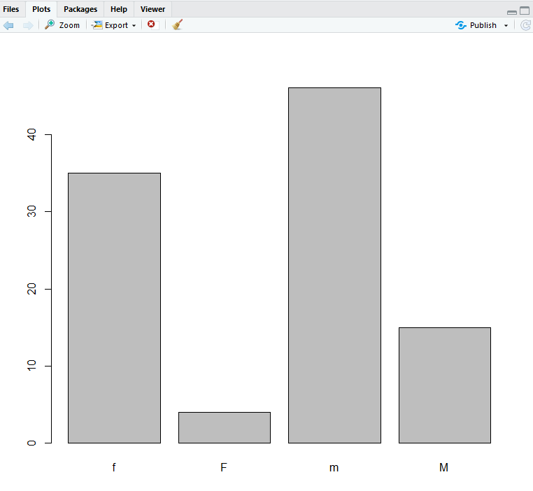
You can even plot a tablle subset:
barplot(table(dat$Gender))

We can definitely see the problem in this column, but how can we fix it? It’s pretty simple really, we just tell R that all the capital “M”’s should be small “m”’s
dat$Gender[dat$Gender=='M']<-'m'
(This R command looks at the column dat$Gender and where the
column dat$Gender equals “M”, we want to give it the new
value of “m”). Then we can plot the dat$Gender
column vs the dat$BloodPressure column.
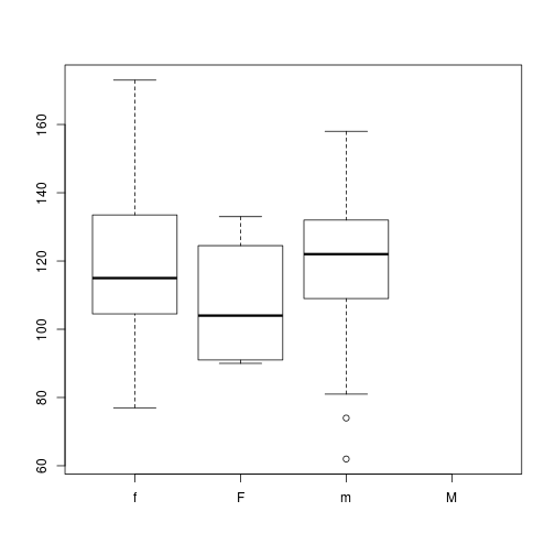
plot(x=dat$Gender,y=dat$BloodPressure)

But something is wrong!! Why does this plot show 4 levels?
Hint how many levels does dat$Gender have?
levels(dat$Gender)
[1] "f" "F" "m" "M"
(Ever heard the expression “Gone but not forgotten”)? This is like that.
Even though we changed all the values of “M” to “m”,
The factor dat$Gender still has the numerical vector,
with value “M” = 0, meaning this level is no
longer used. But to completely eliminate levels from a factor,
we need to explicity tell R that “M” is no longer a
valid value for this column.
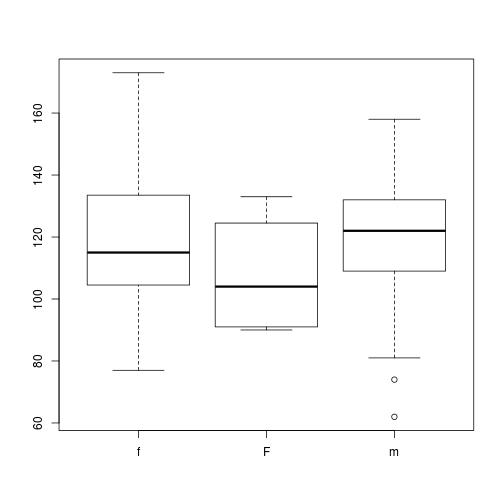
This requires the use of the droplevels() function which
drops unused levels from a factor.
dat$Gender<-droplevels(dat$Gender)
plot(x=dat$Gender,y=dat$BloodPressure)

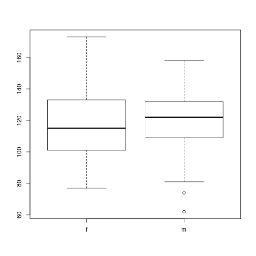
Now you can finish fixing this variable and plot it!
dat$Gender[dat$Gender=='F']<-'f'
dat$Gender<-droplevels(dat$Gender)
plot(x = dat$Gender, y = dat$BloodPressure)

