
Questions
- What will these lessons not cover?
- What are the basic features of the R language?
- What are the most common objects in R?
Objectives
- Be able to create the most common R objects including vectors
- Understand that vectors have modes, which correspond to the type of data they contain
- Be able to use arithmetic operators on R objects
- Understand that lists can hold data of more than one mode and can be indexed
The Pot of Gold…
source("../bin/chunk-options.R")
knitr_fig_path("02-")
Gaining R Competency
Before we begin this lesson, we want you to be clear on the goal of the workshop and these lessons. This is not a course that will “teach you R”. Instead this course is to “teach you enough to use R”. We believe that every learner can achieve competency with R. You reach competency when you find that you are able to use R to handle common analysis challenges in a reasonable amount of time (which includes time needed to look at learning materials, search for answers online, and asking colleagues for help). As you spend more time using R (there is no substitute for regular use and practice) you will find yourself gaining competency and even expertise. The more familiar you get, the more complex the analyses you will be able to carry out, with less frustration, and in less time - the fantastic world of R awaits you!
But, nobody JUST wants to learn R. People want to learn how to use R to analyze their own research questions! Ok, maybe some folks learn R for R’s sake, but these lessons assume that you want to start analyzing genomic data as soon as possible. Given this, we simply won’t have time to cover many valuable R capabilities. But hopefully, we will be giving you just enough knowledge to be dangerous in genomics, which is pretty good in R! We suggest you look into the additional learning materials in the tip box below.
Here are some R skills we will not cover in genomics lessons
- R matrices and R lists
- Loops and conditional statements
- The “apply” family of functions (which are super useful, read more here)
- Basic string manipulations (e.g. finding patterns in text using grep, replacing text)
- Plotting using the default R graphic tools (we will cover plot creation,
but will do so using the popular plotting package
ggplot2) - Advanced R statistical functions
Tip: Where to learn more
The following are good resources for learning more about R. Some of them can be quite technical, but if you become a regular R user you may ultimately need this technical knowledge.
- R for Beginners: By Emmanuel Paradis and a great starting point
- The R Manuals: Maintained by the R project
- R contributed documentation: Also linked to the R project; importantly there are materials available in several languages
- R for Data Science: A wonderful collection by noted R educators and developers Garrett Grolemund and Hadley Wickham
- Practical Data Science for Stats: Not exclusively about R usage, but a nice collection of pre-prints on data science and applications for R
- Programming in R Software Carpentry lesson: There are several Software Carpentry lessons in R to choose from
Creating objects in R
Reminders
At this point you should be coding along in R-studio, using the “genomics_r_basics.R” script we created in the last lesson. Writing your commands in the script (and commenting them) will make it easier to record what you did and why.
What might be called a variable in other computer languages is called an object in R.
To create an object you need:
- a name (e.g. “a”)
- a value (e.g. “1”)
- the assignment operator (“<-“)
In your script, “genomics_r_basics.R”, using the R assignment operator “<-”,
assign “1” to the object “a” as shown. Remember to leave a comment in the line
above (using the #) to explain what you are doing:
# this line creates the object "a" and assigns it the value "1"

a <- 1
Next, run this line of code in your script. You can run a line of code by hitting the Run button that is just above the first line of your script in the header of the Source pane or you can use the appropriate shortcut:

- Windows execution shortcut: Ctrl+Enter
- Mac execution shortcut: Cmd(⌘)+Enter
To run multiple lines of code, you should highlight all the lines you wish to run and then hit Run or use the shortcut key combo listed above.
In the RStudio ‘Console’ you should see:
a <- 1
>
The ‘Console’ will display lines of code run from a script and any outputs or status/warning/error messages (usually in red).
In the ‘Environment’ window you will also get a table:
| Values | |
|---|---|
| a | 1 |
The ‘Environment’ window allows you to keep track of the objects you have created in R. This is very helpful!!!!!
Naming objects in R
Here are some important details about naming objects in R.
- Avoid spaces and special characters: Object names cannot contain spaces
or the minus sign (
-). You can use and underscore (_) to make names more readable. You should avoid using special characters in your object name (e.g.! @ # . ,etc.). Also, object names cannot begin with a number. - Use short, easy-to-understand names: You should avoid naming your objects using single letters (e.g. ‘n’, ‘p’, ‘x’, etc.). This is mostly to encourage you to use names that would make sense to anyone reading your code (a colleague, or even yourself a year from now). Also, avoiding excessively long names will make your code more readable.
- Avoid commonly used names: There are several names that may already have a definition in the R language (e.g. ‘mean’, ‘min’, ‘max’) and these names are reserved. One clue that a name already has meaning (is reserved) is that if you start typing a name, RStudio pops up a colored highlight or RStudio gives you a suggested autocompletion.
- Use the recommended assignment operator: In R, we use
<-as the preferred assignment operator.=works too, but is most commonly used in passing arguments to functions (more on functions later). There is a shortcut for the R assignment operator:- Windows execution shortcut: Alt + -
- Mac execution shortcut: Option + -
There are a few more suggestions about naming and style you may want to learn about as you write more R code. There are several “style guides” that have advice, and one to start with is the tidyverse R style guide.
Tip: Pay attention to warnings in the script console
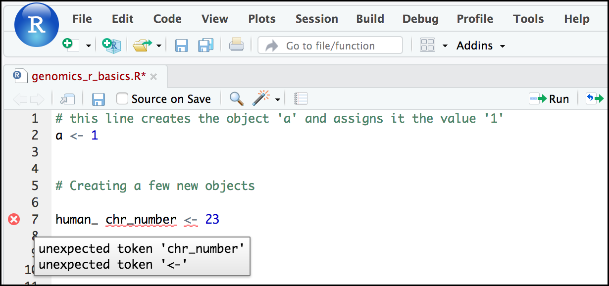
If you enter a line of code in your script that contains an error, RStudio may give you an error message and underline the mistake. Sometimes these messages are easy to understand, but not always. Learning how to properly interpret these warnings will help you find and avoid mistakes. In the example below, our object name includes a ‘space’ character, which is not allowed in R. The error message does not say this directly, but R is telling us something is wrong near
chr_numberor<-. We need to changehuman_ chr_numberto what we wanted:human_chr_number.
Reassigning object names or deleting objects
Once an object has a value, you can change that value by overwriting it. R will not give you a warning or error if you are overwriting an object, which may or may not be a good thing, depending on how you look at it:
# gene_name has the value 'pten' or the value used in the exercise.
# We will now assign the new value 'tp53'
gene_name <- 'tp53'
Now you can see we have changed the value of gene_name by looking at the
“Files/Plots/Packages/Help/Viewer” window of RStudio. Or we could just type
gene_name at the prompt in the consloe window and hit “run”.
You can also remove an object from R’s memory entirely. The rm() function
will delete the object.
# delete the object 'gene_name'
rm(gene_name)
If you then run gene_name, we are told the object no
longer exists.
Error: object 'gene_name' not found
Understanding object data types
In R, every object has two properties:
- Length: How many distinct values are found in that object
- Mode: What is the classification (type) of that object.
Mode
We will get to the “length” property later in the lesson. The “mode” property corresponds to the type of data an object represents. The most common modes you will encounter in R are:
| Mode (abbreviation) | Type of data |
|---|---|
| Numeric (num) | Numbers such floating point/decimals (1.0, 0.5, 3.14), there are also more specific numeric (sub)types (e.g. dbl - Double, int - Integer). These differences are not relevant for most beginners and pertain to how these values are stored in memory |
| Character (chr) | A sequence of letters/numbers in single ‘ ‘ or double “ “ quotes |
| Logical | Boolean values - TRUE or FALSE |
There are a few other modes (e.g. “complex”, “raw” etc.) but “num”, “chr”, and “boolean” are the three we will work with in this lesson.
Data types/modes are common in many programming languages, but also in natural language where we refer to them as the parts of speech, e.g. nouns, verbs, adverbs, etc. Once you know if a word - perhaps an unfamiliar one - is a noun, you can probably make it plural if there is more than one (e.g. 1 Tuatara, or 2 Tuataras). If something is a adjective, you can usually change it into an adverb by adding “-ly” (e.g. jejune vs. jejunely). But context matters; you may need to decide if a word is in one category or another (e.g. “cut” may be a noun when it’s on your finger, or a verb when you are preparing vegetables). These concepts have important analogies when working with R objects.
Here are rules you need to understand about modes in R:
- If you try to assign a series of numbers are given as a value, but they are enclosed in single or double quotes, R will consider them to be in the “character” mode.
- You cannot take a string of alphanumeric characters (e.g. Earhart)
and assign them as a value for an object.
- If you try to assign characters as a value (e.g.:
pilot <- Earhart), it creates an error because R looks for an object namedEarhart(remember that objects have a name AND a value). - Because there isn’t an object currently called
Earhart, no assignment can be made.
- If you try to assign characters as a value (e.g.:
- If we want to create an object called
pilotthat contains the name “Earhart”, we need to encloseEarhartin quotation marks. - If an object called
Earhartalready existed, then the mode ofpilotwould become the same mode as the objectEarhart.
Try this yourself before we move on:
> pilot <- Earhart
Error: object 'Earhart' not found
> Earhart <- "Amelia"
> mode (Earhart)
[1] "character"
> pilot <- Earhart
> mode(pilot)
[1] "character"
> pilot <- "Earhart"
> mode(pilot)
[1] "character"
Did you notice what the object pilot represents now?
Mathematical and functional operations on objects in genomics
Once an object exists (which by definition also means it has a mode), R can appropriately manipulate that object. For example, objects of the numeric modes can be added, multiplied, divided, etc. R provides several mathematical (arithmetic) operators including:
| Operator | Description |
|---|---|
| + | addition |
| - | subtraction |
| * | multiplication |
| / | division |
| ^ or ** | exponentiation |
| a%%b | modulus (returns the remainder after division) |
These can be used with literal numbers:
(1 + (5 ** 0.5))/2
and importantly, can be used on any object that evaluates to (i.e. can be interpreted by R) as a numeric object:
human_chr_number <- 23
# multiply the object 'human_chr_number' by 2

human_chr_number * 2
Vectors
Vectors are probably the
most used commonly used object type in R.
A vector is a collection of values that are all the same mode (numbers, characters, etc.).
One of the most common
ways to create a vector is to use the c() function - the “concatenate” or
“combine” function. Inside the function you may enter one or more values; for
multiple values, separate each value with a comma:
# Create the SNP gene name vector

snp_genes <- c("OXTR", "ACTN3", "AR", "OPRM1")
Vectors always have a mode and a length.
You can check these with the mode() and length() functions respectively.
Another useful function that gives both of these pieces of information is the
str() (structure) function.
# Check the mode, length, and structure of 'snp_genes'
mode(snp_genes)
length(snp_genes)
str(snp_genes)
Vectors are quite important in R. Another data type that we will work with later in this lesson, data frames, are collections of vectors. What we learn here about vectors will pay off even more when we start working with data frames.
The magic of programming
To understand why the expression
snp_positions[snp_positions > 100000000]
works you need to examine how R evaluates the expression
snp_positions > 100000000.
snp_positions
[1]   8762685  66560624  67545785 154039662
snp_positions > 100000000
[1] FALSE FALSE FALSE  TRUE
The output above is a logical vector, the 4th element of which is TRUE. When you pass a logical vector as an index, R will return the all TRUE values. You can even tell R to return any value, if you assign it a logical value of “TRUE”:
snp_positions[c(FALSE, FALSE, FALSE, TRUE)]
[1] 154039662
snp_positions[c(FALSE, FALSE, TRUE, FALSE)]
[1] 67545785
If you have never coded before, this example starts to expose the “magic” of programming. We mentioned before that with bracket notation you use a named vector followed by brackets which contain an index:
named_vector[index]
The “magic” is that indexes evaluate to a number. So, even if the indexed values are not integers, R can evaluate the vector indexes and that allows us to get a result!
One more example:
To show that our expression
snp_positions[snp_positions > 100000000] evaluates to a number.
If you wanted to know which index
(1, 2, 3, or 4) in our vector of SNP positions is the one greater than
100,000,000 we can use the which() function to return the indices
of any item that evaluates as “TRUE” in our comparison:
which(snp_positions > 100000000)
[1] 4
Why this is important
Often in programming we are working with values, but for our code to be flexible, it needs to be able to accept whatever value is input, or output, when executing the next piece of code. Rather than always putting in a pre-determined value (e.g 100000000) we can use an object that can take on whatever value the code needs. So for example:
snp_marker_cutoff <- 100000000
snp_positions[snp_positions > snp_marker_cutoff]

# Now ANY SNP positions greater than 100000000 are
# the returned value!!!!!
Now you can begin to see that when the value for
snp_marker_cutoffchanges, it changes throughout the lines of code.
Ultimately, putting together flexible, reusable code like this gets at the “magic” of programming!
A few final vector tricks
Finally, there are a few other common retrieve or replace operations you may
want to know about. First, you can check to see if any of the values of your
vector are missing (i.e. are NA). Missing data will get a more detailed treatment later,
but the is.NA() function will return a logical vector, with “TRUE” for any NA
value:
# The current value of 'snp_genes':
snp_genes
[1] "OXTR" "ACTN3" "AR" "OPRM1" "CYP1A1" NA "APOA5"

is.na(snp_genes)
[1] FALSE FALSE FALSE FALSE FALSE  TRUE FALSE
Sometimes, you may wish to find out if a specific value (or several values) is
present in a vector. You can do this using the comparison operator %in%, which
will return “TRUE” for any value in your collection that is in
the vector you are searching:
# current value of 'snp_genes':
snp_genes
[1] "OXTR" "ACTN3" "AR" "OPRM1" "CYP1A1" NA "APOA5"

# test to see if "ACTN3" or "APO5A" is in the snp_genes vector
# if you are looking for more than one value, you must pass this as a vector

c("ACTN3","APOA5") %in% snp_genes
[1] TRUE TRUE
Keypoints
- “Effectively using R is a journey of months or years.” *
You don’t have to be an expert to use R and you can start using and analyzing your data with about a day’s worth of training. Review this lesson whenever starting an R analysis. - It is important to understand how data are organized by R in a given object type and how the mode of that type (e.g. numeric, character, logical, etc.) will determine how R will operate on that data.
- Working with vectors effectively prepares you for understanding how data are organized in R.
* François Michonneau, May, 2019, Genomics Workshop Bug BBQ, Univ. of Arizona, Phoenix, AZ