(This workshop-style lesson is being taught on the Pete supercomputer at OSU)

Hands-on Genome Assembly Reporting

A contig is a contiguous length of genomic sequence (an individual piece of a genome). A scaffold is composed of ordered contigs and gaps. Scaffolding generally relies on a reference genome, that can be used to “map” the location of each contig, placing them in the correct order (and by definition creating “scaffolds”).

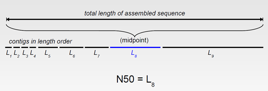
By far the most widely used statistics for describing the quality of a genome assembly are its scaffold and contig N50s. A contig N50 is calculated by first ordering every contig by length from longest to shortest. Next, starting from the longest contig, the lengths of each contig are summed, until this running sum equals one-half of the total length of all contigs in the assembly. The contig N50 of the assembly is the length of the shortest contig in this list. The scaffold N50 is calculated in the same fashion but uses scaffolds rather than contigs. The longer the contig or scaffold N50 is, the better the assembly is. However, it is important to keep in mind that a poor assembly may have forced unrelated reads and contigs into scaffolds creating an erroneously large N50.

Another way to say this is the N50 statistic is a metric of the length of a set of sequences. N50 is the contig length such that using equal or longer contigs produces half the bases.

Think of it as the contig in the middle when all contigs are lined up by size. The size of that contig, is the N50 size.

Maybe a figure will help.

Now that we have completed several assemblies, let’s look at our results. Change to the results directory and list the files. The output should look similar to the file list below:

$ cd ../../results
$ ls
spades21.fasta  spades31.fasta  velvet31.fasta
spades25.fasta  quast.sbatch  velvet21.fasta  velvet25.fasta

These files are the results from all the programs using different K-mer parameters. If you have a different assembly (e.g. different K-mers) using the same assembler, make sure you name them differently, but consistently. For example: spades29.fasta spades33.fasta velvet39.fasta

_____________`

Validation

Make sure that you validate the results before releasing it. Some assemblies may appear to have large contigs and scaffolds, but are wrong. Check the assembly!

We are going to evaluate our assemblies with quast.py.

Downloading QUAST

From the mcbios directory enter the following command:

wget https://github.com/ablab/quast/releases/download/quast_5.0.2/quast-5.0.2.tar.gz

This will download the quast-5.0.2.tar.gz file. To uncompress it use the command:

tar -xvzf quast-5.0.2.tar.gz

You should now have a subfolder named quast-5.0.2. Now change to the results directory below the mcbios directory. Use nano to look at the quast PBS submission script.

$ nano -w quast.sbatch

The file looks like this:

#!/bin/bash
#SBATCH -p express
#SBATCH -t 1:00:00
#SBATCH --nodes=1
#SBATCH --ntasks-per-node=1
#SBATCH --mail-user=peter.r.hoyt@okstate.edu
#SBATCH --mail-type=end

export GROUPNUMBER=1
export DATADIR=../data/group${GROUPNUMBER}

../quast-5.0.2/quast.py --gene-finding  `ls *.fasta`  -o quastresults  -R ${DATADIR}/ref.fasta

When you are ready to run quast, remember to change your groupnumber. The quast.sbatch will analyze all the *.fasta files in your results directory.

Submit the quast.sbatch file:

$ sbatch quast.sbatch

When quast is finished look at the output file to check for obvious errors.

$ less slurm<jobid>.out (protip: use TAB autocomplete so you don’t have to type in the jobid)

You may see some warnings that quast could not find genes, or that some images could not be created. That’s okay. Quast can do a lot of things we aren’t validating today. If there are no fatal errors, press q to exit the less command. Now you can send everything to yourself.

Before we send everything, we will zip the entire quast directory. It’s good practice to compress files when transferring them because they transfer faster, and the use less bandwidth. After the zip command is complete, we can use scp to transfer the file to our desktop!

$ cd ..
$ zip -r quast.zip quastresults

Now switch to your Gitbash Window and from there make sure you are on your Desktop by typing cd ~/Desktop

Then (using your own username) download the quast results by typing:

$ scp phoyt@pete.hpc.okstate.edu:/scratch/phoyt/mcbios/results/quast.zip .

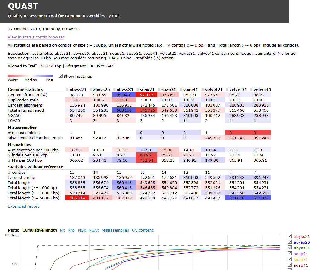
When the quast.zip file is on your Desktop, extract the file, and double-click on the report.html file to open it in your browser. If the file doesn’t open, your browser may need Javascript to be enabled. Note that this html web page is interactive! You should see something like the image shown below, except we are only using two Assemblers; velvet and SPAdes:

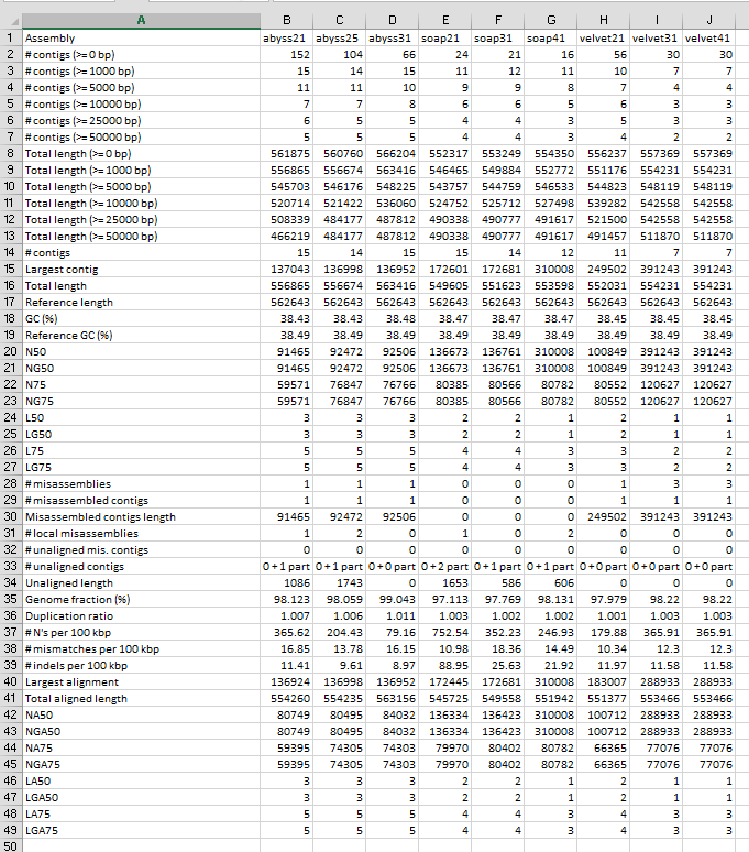
Before we cover information in the web page, notice that the report results are also available as report.pdf, and the file report.tsv (and report.txt) are tab-delimited text files that will open in a spreadsheet as shown below for Group2. Quast is useful software!

We are going to look at the quast report.html file because it contains almost all the data that you’ll find in the other files. This web page shows you the analysis of each assembly you made. You can now compare the assemblies based on good or bad qualities of the assembly statistics. This is an important moment for you as a bioinformatician, because it’s up to you to determine which assembly is the best, and why.

And there is a problem: it isn’t always a clear which assembly is the best. It may depend on how you set up the experiment, and what you were trying to identify in the assemblies.

But there are some rules we can use:

1. Misassembled genomes are very bad.
2. Indels (Insertions or Deletions) are very bad.
3. Runs of N or lots of Ns are bad (but fixable)
4. Genome sizes that are close to the reference genome size are good (but can be wrong).
5. Large N50 scores are good (but the largest isn’t always the best).
6. Combinations of bad things make the assembly worse.
7. Combinations of good things make the assembly better.

Before you make a decision, click on the blue letters that say Extended report. Now you have a lot more information! Notice you can hover your mouse over the row identifiers (column1) and a description will pop up. Spend about 5 minutes (or more if you are doing this at home) and check out all the information Quast has given you to help you decide if your assemblies are good. When you are done, use the Quast manual to get answers to the following question:

Which assembly has better length statistics?

Best assembly: _________________

Worst assembly: _________________

How does your assembly compare structurally to the reference genome?

Icarus Browser

There’s even more data to explore! Click on the “View in Icarus contig browser” link under the date near the top of the Quast web page. You should now see a graphical rendetion of your aligned genomes. This is a lot of information!

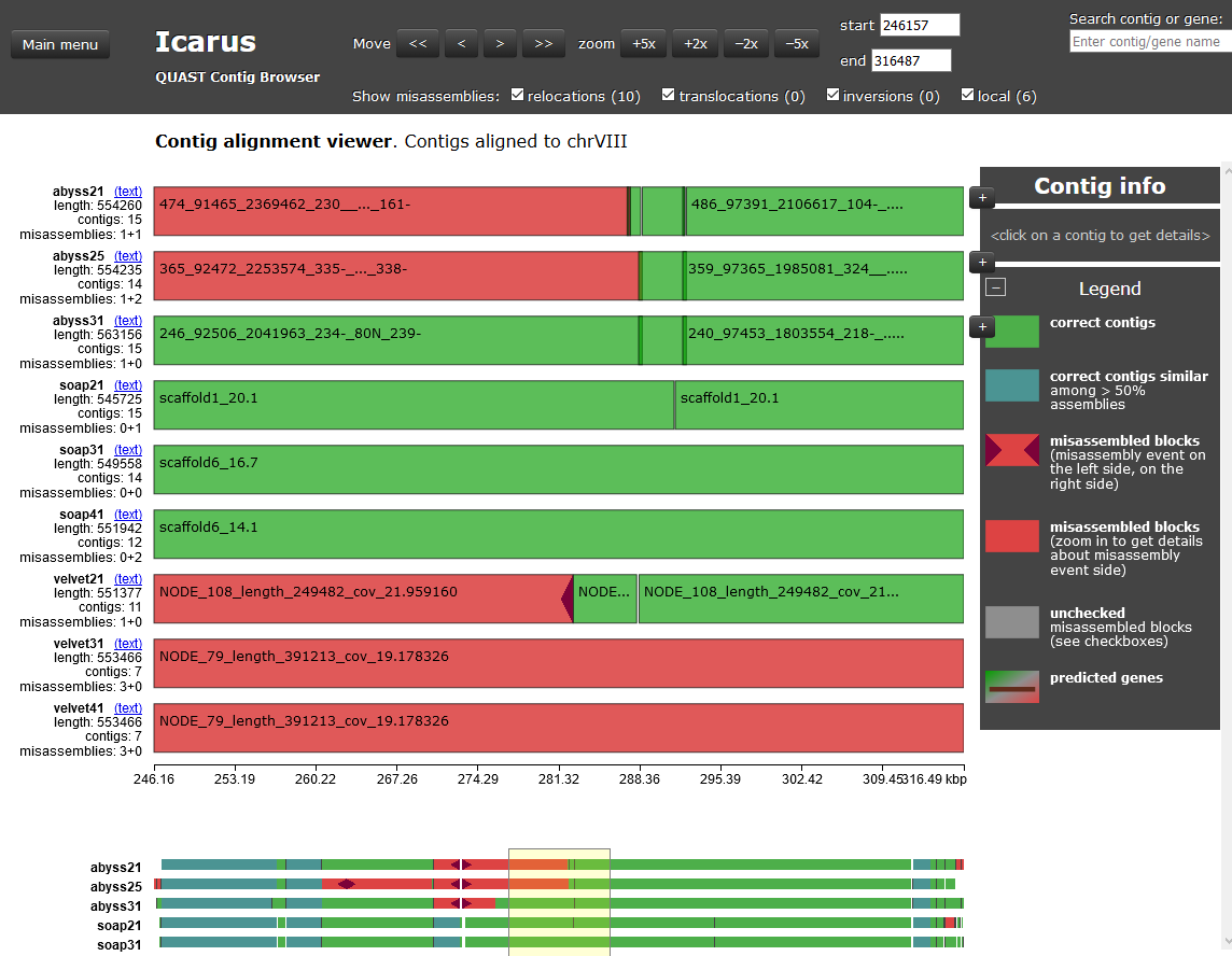
Additionally, if you click on the button at the top left that says “Main menu” you’ll be able to choose between the “Quast report”, or the “Contig alignment viewer” (the previous page) or the “Contig size viewer” (The Contig size viewer should make it easier to eliminate some of the assemblies).

SORRY! BUT THIS IS TOO MUCH

Because we don’t have time to go over all these data with you. We are only showing you that you can do this! Spend some time going over everything revealed in these charts. Make new assemblies and put them into your results directory and re-run Quast. Check out the Quast manual again. You should be curious, and that’s good.

Re-aligning

It is very common that figuring out which is the best assembly is hard. But you can eliminate some of the assemblies based on misassemblies or indels. Once you have eliminated some assemblies you can go back and try more K-mer values!

Re-aligning is a very good idea when you are first starting to assemble genomes. Some bioinformaticians prefer to re-align their own best assemblies using even more (different) software.

EXTRAS:

Congratulations!

You have learned a lot about genome assembly and are using your skills in the bash shell to run real data. It’s always good to appreciate these small victories in science.

Below we present some additional bioinformatics software on Pete that you might want to try. Although the commands are not exactly the same as those used in our lesson, you should be able to read the manuals, and figure out the commands to run these software on our example files. Some of these software are pipelines that include the software we have experimented with today.

http://kmergenie.bx.psu.edu/ “kmergenie”

Another de novo assembly tutorial: http://www.cbs.dtu.dk/courses/27626/Exercises/denovo_exercise.php (uses quake & jellyfish)

good outline: http://en.wikibooks.org/wiki/Next_Generation_Sequencing_(NGS)/De_novo_assembly

github repostiory with lots of slides etc: https://github.com/lexnederbragt/denovo-assembly-tutorial

(Acknowledgment: This exercise was originally presented at OSU by Dr. Haibao Tang, JCVI (now an independent consultant). It was modified by Dr. Dana Brunson, OSU HPCC (now at Internet2), and Dr. Peter R. Hoyt, OSU Biochemistry and Molecular Biology)